Introduction

Pardon the dust, this is being rewritten.

These notes are on the COP3530 Data Structures and Algorithm class with the excellent Professor Kapoor at the University of Florida as well as on Abdul Bari’s DSA Course on Udemy . What I have learned from each has been compounded into one living document. If you are interested in Abdul Bari’s course but want a bit of a taste for it, there is also a free YouTube version that is consolidated . Please note that these are notes, I can’t stress this enough. These are written with prior knowledge in mind, and are basically useless if you aren’t following along with a textbook or a course. They won’t be teaching you well. These can act as a good reference for concepts and important explanations. Think of it as a TL;DR on things, but you’re doing yourself a disservice if you even think of using these as your main source of info. For textbooks, check out the excellent OpenDSA Book . If you prefer paper, check out “Introduction to Algorithms” by Cormen & Leiserson and “Data Structures and Algorithm Analysis in C++" by Weiss.

Definition of the Data Structure and the Algorithm

• What is a Data Structure?

  • A data structure can be defined as the arrangement of a collection of data items so that they can be utilized efficiently. It is all about data and the operations of the data.

• What is an Algorithm?

  • An algorithm can be defined as a procedure used for solving a problem or performing a computation. It is a finite set of instructions to execute a task. All algorithms have an input, an output, and are definite and unambiguous. This means that they always have the same output for a given input.

Algorithm vs. Program

Algorithms focus more on how to solve versus programs which is how we implement the solution.

Multiple Solutions to a Problem

The proverb “more than one way to skin a cat” holds very true here, and there is definitely some more efficient ways to solve a problem. This is the difference between solutions, some are naïve, or silly, whereas others are more artful, or better. For instance, imagine we are given this objective:

• Determine if a sorted array contains any duplicates.

One possible solution is to compare every element to every other following element so as to create pairs, and if a pair shares identical elements, then there is a duplicate. The issue with this solution is that it is not taking full advantage of the characteristics of the data it has been given. Note that this array is sorted. This means that another, much better solution, is to compare each value with the value immediately proceeding it. Because it is sorted, duplicates will be right next to each other! Each solution yields the same result, but our latter solution is much more efficient. So this yields a very important question? Are all algorithms equal in terms of performance? And if not, how do we evaluate performance in a meaningful way?

What is Performance and Why Should We Care?

Performance for algorithms is defined in terms of time and space. These will be discussed later. Algorithm analysis is important for a few reasons. For one, it allows us to think critically about what we are creating, and as a result allows us to find the best solution to a problem. It also allows us to sell a product, if we can boast that our product is the best because of its performance, it’ll sell more. Performant algorithms also cost less to run, it might seem negligible at first, but faster algorithms save time, and time is money. In some cases, a solution to an issue with certain data sets can take 30 seconds, or a year.

How to Measure Performance?

It is great that we know the importance of performance, but what are some ways that we can truly understand performance in a meaningful way?

Different Approaches of Measurement

Approach 1: Simulation with Timing

A logical way of checking performance is to just time two solutions, and then compare the times.

Code #1:

1
2
3

auto t1 = Clock::now();
for (int i=0; i < 1000; i++);
auto t2 = Clock::now();

Code #2

1
2
3

auto t1 = Clock::now();
for (long i = 0; i < 1000000; i++);
auto t2 = Clock::now();

Looking at the difference between t2 and t1 for each snippet:

• Code 1: 1873 nanoseconds
• Code 2: 1644295 nanoseconds

The pros of timing is that it is easy to measure and interpret. The cons are that results vary across machines, compilers, and implementations. It isn’t predictable for smaller inputs. There isn’t a clear relationship between input and time.

Approach 2: Modeling by Counting

Instead of counting time, we count the number of operations there are:

1
2
3
4

int sum = 0;
for (int i = 0; i < n; i++)
    sum += i;
std::cout << sum;

The pros of counting is that it is independent of the computer and its input dependence is captured in modeling. The cons is that there is no formal definition of which operation to count, and it is tedious to compute. Also results still vary across implementation and it doesn’t really tell you the time.

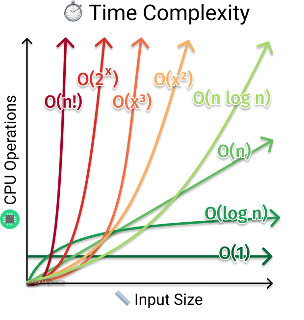
Approach 3: Asymptotic Behavior: Order of Growth

An order of growth are functions whose asymptotic behavior is seen as equivalent. For example, $8n$, $100n$, and $n + 1$ all fall into the same order of growth, $n$. The major order of growths that algorithms follow with inputs are:

This can be further illustrated by:

Sourced from Adrian Mejia

So if we return to the example in Approach 2, we note that $T(n) = 3n + 4$. How would we express the time complexity of this algorithm utilizing order of growth? This can be done with the Big O notation, which represents the upper bound of a function’s growth rate. There are other notations that describe other aspects of a function, but for the sake of algorithm performance, Big O is usually what is considered. In this way, Big O notation represents the worst case of an algorithm. Let’s look at how these notations are formally defined and how to use them to describe the performance of an algorithm.

Asymptotic Analysis (Time Complexity)

Asymptotic Analysis (aka. asymptotics) is a mathematical method to describe the limiting behavior of functions. For instance, imagine we are considering a function $f(x) = x^2 + 3x$, as $x \rightarrow \infin$, the term $3x$ becomes more and more insignificant when compared to the term $x^2$. In this way, it is said that $f(x)$ is asymptotically equivalent to $x^2$ as $x \rightarrow \infin$. In Computer Science, we are especially interested in asymptotic analysis because it allows us to analyze algorithms in a meaningful and quantifiable way.

Notation

Big O

Let $T(n)$, $f(n)$ be functions. Therefore, $T(n) \in O(f(n))$ if there exists two positive constants $n_0$ and $M$ such that $T(n) \le Mf(n)$ for all $n \ge n_0$. Formally speaking, this is a more restrictive definition that is of most concern to us as Computer Scientists, but if you are interested in other definitions check out the formal definition for Big O notation here. With this definition, a function $T(n) = n$ will yield $T(n) \in O(n!)$, but although true, isn’t terribly useful. As a result, when figuring out the Big O of a function, it is best to figure out the tightest upper bound, so in the previous case, $T(n) \in O(n)$. Taking a look at our example from Approach 2, $T(n) = 3n+4$. When considering this, what should the value $M$ be? The easiest way to do this is to set $M$ to equal each of the integers in the function, so $M = 3 + 4 = 7$, and we set $n_0 = 0$. So, $3n+4 \le 7n$ for all $n > 1$, so $T(n) \in O(n)$. The function $f(n)$ always acts as an upper bound on performance, and $T(n)$ will grow no faster than the constant $M$ times $f(n)$.

Big Ω

Let $T(n), g(n)$ be functions. Therefore, $T(n) \in \Omega(g(n))$ if there exists two positive constants $n_0$ and $M$ such that $T(n) \ge Mg(n)$ for all $n \ge n_0$. Similar to Big O, this means that when $T(n) = n^3$, $T(n) \in \Omega(1)$, but that isn’t useful. So, whenever you figure out the Big Ω of a function, find the tightest lower bound, so in the previous case, $T(n) \in \Omega(n^3)$. The function $g(n)$ always acts as a lower bound on growth rate of $T(n)$, and $T(n)$ will grow no slower than the constant $M$ times $g(n)$.

Big Θ

Let $T(n), g(n)$ be functions. Therefore, $T(n) \in \Theta(g(n))$ if $T(n) = O(g(n))$ and $T(n) = \Omega(g(n))$. Another way of expressing it is $T(n) \in \Theta(g(n))$ if there exists two positive constants $n_0$ and $M$ such that $Mg(n) \le T(n) \le Mg(n)$ for all $n \ge n_0$. This function represents the upper and lower bound on the growth rate of $T(n)$.

Rules

The rules for Asymptotic Analysis are pretty simple, but are incredibly important to learn.

1. Addition (Independence): $T(n) = O(n+m)$

Given different parts of an algorithm, their time complexities can be added:

1
2
3
4
5
6
7
8

void my_function(int n, int m)
{
  for (int i = 0; i < n; i++)
    // Do stuff

  for (int i = 0; i < m; i++_
    // Do more stuff
}

The time complexity of lines 3 and 4 is $O(n)$ and the time complexity of lines 6 and 7 is $O(m)$, the time complexity for this algorithm is $O(n+m)$

2. Drop Constant Multipliers: $T(n) = O(n+n) = O(2n) = O(n)$

Given the following algorithm:

1
2
3
4
5
6
7
8

void my_function(int n)
{
  for (int i = 0; i < n; i++)
    // Do stuff

  for (int i = 0; i < n; i++_
    // Do more stuff
}

Lines 3 and 4 is $O(n)$ and lines 6 and 7 are $O(n)$, which is $O(n+n) = O(2n) = O(n)$

3. Always Differentiate Input Variables

Using the algorithm from Rule #1, we would never write the time complexity as $O(n)$ or $O(m)$, but always $O(n + m)$ unless there is an indication of a relationship between the variables given.

4. Dropping Lower Order Terms

Given the following algorithm:

1
2
3
4
5
6
7
8

void my_function(int n, int m)
{
  for (int i = 0; i < n; i++)
    // Do stuff

  for (int j = 0; j < m; j *= 2)
    // Do stuff
}

Lines 3 and 4 is $O(n)$ and lines 6 and 7 are $O(log_2 m)$, thus the time complexity for this algorithm is $O(n + log_2 m)$. Now, if we were told that $n$ and $m$ grow at the same rate, then $O(n + log_2 m) = O(n)$. This is because we drop the lowest order term whenever variables grow at the same rate, or they are identical variables.

Cases

Algorithms that have a purpose that allows them to stop their process (e.g.. searching algorithms, they stop once they find what they are looking for) due to a condition have different cases. These are the best case, average case, and worst case. The best case is the lowest cost, average case is the average cost for all n, and worst case is the highest possible cost.

Recursion

Introduction

A small topic detour for a concept that is valuable to understand in a DSA class, which is recursion. There are a lot of different types of recursive functions, and understanding how they are used is important. Let’s take a look at how recursion works and how we define it.

Given the function fun(int n):

1
2
3
4
5
6
7
8
9

int fun(int n) {
  if (n > 1)
  {
    return fun(n-1) * 2;
  } else
  {
    return n;
  }
}

We can see that the function consists of an if-else statement, where if the input is greater than 1, we return the value of the function fun(n-1)*2, and if not, we just return n. In this way, we can simplify the function to just be:

1
2
3
4
5
6
7

int fun(int n) {
  if (n > 1)
  {
    return fun(n-1) * 2;
  }
  return n;
}

This is an example of a recursive function. A recursive function consists of two parts, an ascending portion and a descending portion. We ascend by returning values of the function, and descend once we reach our catch value, in this case it is once $n \le 1$. The algorithm returns $2^n$.

Tail Recursion

Tail recursion is defined as recursion in which the last statement is the recursive call, for example:

1
2
3
4
5
6
7
8

void fun(n) {
  if (n > 0)
  {
    // Do stuff Here
    // ...
    fun(n-1);
  }
}

So all the processing is done before the recursive call.

Head Recursion

Head recursion is defined as recursion in which the first statement is the recursive call, for example:

1
2
3
4
5
6
7
8

void fun(n) {
  if (n > 0)
  {
    fun(n-1);
    // Do stuff Here
    // ...
  }
}

So all the processing is done after the recursive call.

Linear Recursion vs. Tree Recursion

Linear Recursion is recursion in which there is only one branch of recursion, in other words it maintains a straight line, for example:

 1
 2
 3
 4
 5
 6
 7
 8
 9
10

void fun(n) {
  if (n > 0)
  {
    // Do stuff hereLR
    // ...
    fun(n-1);
    // Do stuff here
    // ...
  }
}

Tree Recursion is recursion in which there is more than one branch of recursion, kind of like a tree, for example:

 1
 2
 3
 4
 5
 6
 7
 8
 9
10
11
12
13

void fun(n) {
  if (n > 0)
  {
    // Do stuff here
    // ...
    fun(n-1);
    // Do stuff here
    // ...
    fun(n-1);
    // Do stuff here
    // ...
  }
}

An example of tree recursion can be found here:

 1
 2
 3
 4
 5
 6
 7
 8
 9
10

#include <stdio.h>

void fun(int n) {
  if (n > 0)
  {
    printf("%d ", n);
    fun(n-1);
    fun(n-1);
  }
}

This will give the output 3 2 1 1 2 1 1. This is because we call the function with the input 3, we print 3, and then call fun(3-1), it then prints 2, and then calls fun(2-1), which prints 1, and then calls fun(2-1) again, which prints 1. Then we descend, and fun(3-1) is called a second time, which repeats the same process over again one last time.

Indirect Recursion

Indirect recursion is recursion that happens between two or more functions, which makes a sort of circular pattern, for example:

 1
 2
 3
 4
 5
 6
 7
 8
 9
10
11
12
13
14
15
16

void A(int n) {
  if (<-->)
  {
    // Do stuff here
    // ...
    B(n-1);
  }
}
void B(int n) {
  if (<-->)
  {
    // Do stuff here
    // ...
    A(n-1);
  }
}

Nested Recursion

Nested Recursion is recursion within recursion, in other words a recursive call within a recursive call, for example:

1
2
3
4
5
6
7

void fun(int n) {
  if (<-->)
  {
    // Do stuff here
    fun(fun(n-1));
  }
}

In this way, we evaluate the parameter of the recursive call first, then whatever that is, place it into that recursive call.

Examples of Recursion

Fibonacci Sequence

The Fibonacci Sequence is defined as $F_n = F_{n-1} + F_{n-2}$, where $F_0 = 0$ and $F_1 = 1$. We can use Tree Recursion to write an algorithm to calculate the sum of the sequence:

1
2
3
4
5
6
7

int fib(int n) {
  if (n <= 1)
  {
    return n;
  }
  return fib(n-1) + fib(n-2);
}

Sum of Natural Numbers

The sum of all natural numbers at point n, is equal to the sum of the natural numbers $(n-1)$, plus $n$. In other words, sum(n) = sum(n-1)+n

 1
 2
 3
 4
 5
 6
 7
 8
 9
10

int sum(int n) {
  if (n == 0)
  {
    return 0;
  }
  else
  {
    return sum(n - 1) + n;
  }
}

Abstract Data Types and Linear Ordered Data Structures

What is an Abstract Data Type?

An Abstract Data Type (ADT) is a Data Type where the operation is known, but the representation is not. A real life example is a book, a book is Abstract, but a Telephone Book is a representation. We will look at all of these Logical Data Structures as ADT first, so we can understand them, and then we can delve into how they work. This means that an Abstract Data Type acts as a mathematical or logical model of a way to store and organize data. They are basically a class of objects whose logical behavior is defined by a set of values and operations. We define the data and the operations, but we don’t care about the implementation. This is the opposite of a concrete data type consists of its representation and its operation. The representation is what it actually is and how it is implemented. The operation portion is what can be done with the data. In other words, the representation is the technical details of a data type, and the operation is what we can actually do with it.

An example of an ADT is a list. A concrete data type (e.g.. implementation) of list is an array, linked list, vector, etc.

Linear Ordered Data Structures

List ADT

Core features:

• Ordered collection of data (e.g.. all elements have an ordered positive.)
• Linear Structure.
• Can have a size, it can grow and shrink.
• Can store any element type (i.e isn’t limited to a single type of data.)

The list basically is just one value after another, e.g.. 1, 2, 3, 4, etc. It is linear, meaning it goes forwards and backwards.

Characteristics:

• Data

  • Items
  • Current number of items stored
  • Capacity, is it bounded to a maximum?

• Operations

  • Read, Write, and Remove elements.
  • Find an element.
  • Count the number of elements.
  • Traverse the list.

Array Implementation

Characteristics

• They have a fixed size
• Stores similar elements (store the same or similar types)
• Contiguous indices (e.g.. $0, 1, 2…n-1$)
• Elements are stored contiguously in memory.
• Allows for random access, given an indice you can access the element there (e.g.. Array[n])

Operation Performance

To add or remove anything from the beginning, it requires shifting $n$ elements to the right, resulting in $O(n)$. Similar is true for the middle, but instead shifting all elements to the right of the indice being considered. This is still $O(n)$ because this indice grows with $n$. In the case of the end, it is constant because the size of the array is known, and this means that it is free to add and remove from the end of it (i.e. no shifts are required.)

• Benefits
  • Constant access time, Array[i] = arr + (i * sizeOf(type)).
  • Constant time for adding and removing elements from the end.
• Drawbacks
  • Expensive for adding and removing elements from the beginning or middle.

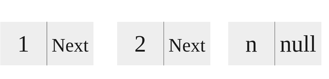
Singly Linked List Implementation

A diagram of a Singly Linked List

Each of these elements are called a Node. A Node contains an element and a pointer to another Node. This goes on and on until the pointer points to a nullptr (i.e. points to nothing.) An example Node object in C++ would look like this:

1
2
3
4
5
6
7
8
9

#include <iostream>

template <typename T>
class Node
{
  public:
    Node* next;
    T data;
}

In this instance, a Node contains the pointer to the next Node as well as the data of some type T. This can be used like this:

1
2
3

Node<int>* node_one = new Node<int>();
node_one->data = 10;
node_one->next = nullptr;

We can also design a constructor for Node:

 1
 2
 3
 4
 5
 6
 7
 8
 9
10
11
12

Node::Node(T data, Node* next)
{
  this->data = data;
  this->next = next;
}

int main()
{
  Node<int>* my_list = new Node<int>(10, nullptr);
  my_list = new Node<int>(20, my_list);
  my_list = new Node<int>(30, my_list);
}

Thus this list is represented as:

1

30 -> 20 -> 10 -> /

In this case, the length of this list is one.

The Node class works great, but it is a bit verbose. In actuality, the list requires a lot more features than this, we are just describing everything manually. In this case, encapsulating Node by another class is much better.

 1
 2
 3
 4
 5
 6
 7
 8
 9
10
11
12
13
14
15
16
17
18
19
20
21
22
23
24
25
26
27
28
29
30
31
32

template <typename T>
struct Node
{
  T data;
  Node<T> *next;
}

template<typename T>
class List
{
  private:
    int size;
    Node<T> *head;
    Node<t> *tail;

  public:
    List()
    {
      size= 0;
      head = new Node<T>;
      tail = new Node<T>;
      head->next = tail;
    }

    void push_front(T element)
    {
      Node<T> *q = new Node<T>;
      q->data = element;
      q->next = head->next;
      head->next = q;
    }
}

With this example, our linked list contains two nodes, the head and the tail. In this implementation, these are sentinel nodes, which basically represent the path entry and the path terminator. Don’t worry much about them. In this example, our push_front operation creates a new Node with element, and then changes the Node’s next to be whatever the head is pointing to next. Then we change the head next to be our new Node q. To visualize this:

1
2
3
4
5

Before calling push_front:
H -> T

After calling push_front:
H -> q -> T

Where q is our new node.

Characteristics

• Consists of Nodes
  • Data
  • Pointer to a following Node
• Stores similar elements (i.e. stores all of the same type.)
• Elements are linked in memory but are stored non-contiguously.
• Doesn’t allow for random access

Operation Performance

• Add - PushFront(key), PushBack(key)
• Remove - PopFront, PopBack
• Get - TopFront, TopBack
• Find(key), Erase(key), Empty()
• AddBefore(Node, key), AddAfter(Node, key)

Performance of these operations

• Benefits
  • Adding and Removing in front is way faster, $O(1)$
• Drawbacks
  • Expensive random access, $O(n)$
  • TopBack, PushBack, PopBack, and AddBefore are also very expensive
  • More expensive in terms of memory

Improving Singly Linked List with Tail

By adding a true tail pointer (eg. it points to the back most element.) You can improve the PushBack and the TopBack performance to be $O(1)$. This significantly increases the usefulness of the singly linked list immensely. The issue is that PopBack and AddBefore is $O(n)$. Is there anyway to improve this? There in fact is.

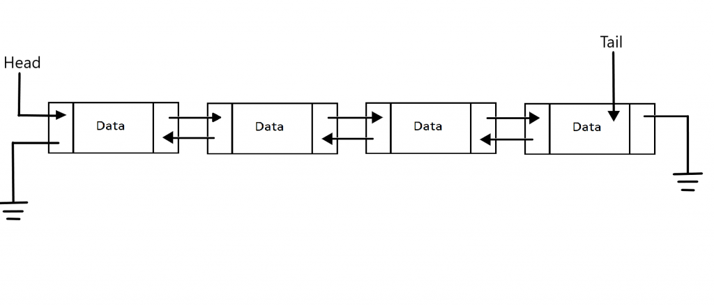
Doubly Linked List with Tail Implementation

Sourced from AskPython

In this type of linked list, a Node contains a pointer to a previous element, the current data of some type, and the following elements. This means that from any Node, you can go forwards and backwards. This means that Node looks something like:

1
2
3
4
5
6
7

template <typename T>
struct Node
{
  Node<T> *prev;
  T data;
  Node<T> *next;
}

Furthermore, this solves the issue of PushBack, PopBack, TopBack, and AddBefore, all of which are now $O(1)$ time complexity instead of $O(n)$. The trade off is that this implementation requires extra memory. This is because this list implementation has access to the tail. When we have access to the tail and the have a pointer in both directions, we can view the tail, append to the tail, and AddBefore the tail (as well as any Node.) Let’s take a look at how some of this logic looks. Whenever we want to remove a value before the tail in this given doubly linked list:

1
2

H -> 2 -> 3 -> T
  <-   <-   <-

Let’s say we want to remove 3, in this case we’d access the tail value. We’d set tail->prev->prev->next = tail, and then set tail->prev = tail->prev->prev. We would also throw in a delete somewhere to make sure we are deleting the old node:

1
2

H -> 2 -> T
  <-   <-

Circular Linked List

I won’t go into these as they aren’t exactly needed to be known in this class, but basic things should be understood. Just check out this GeeksForGeeks article on Circular Singly Linked Lists as well as this one on Circular Doubly Linked List .

Array vs. Linked List

In terms of Space, there are two things, List size and Element size.

• List Size, in Linked List favor
  • In the array implementation, an estimate of the size when the list is created is required, and when this size is met, the array must be reallocated.
  • In the linked list implementation, the size is dynamic and can grow as needed.
• Element Size, in Array favor
  • In the array implementation, only the element is needed to be stored.
  • In the linked list implementation, it requires storage for the element as well as pointer(s).

In terms of Time, there are two things, access as well as adding and removing.

• Access, in Array favor

  • In the array implementation, values can be randomly accessed in constant time at any index.
  • In the linked list implementation, values must be accessed by traversing the list one element at a time.

• Adding and Removing, in Linked List favor

  • In the array implementation, it requires all elements to be moved whenever we add or remove from the array.
  • In the linked list implementation, insertion and removal is constant time if the iterator is where you need it to be.

STL Lists

The C++ Standard Template Library contains 4 major list implementations. The Forward_list which is Singly Linked List implementation. The List which is a doubly linked list implementation. The Array which is a fixed size list. Finally, Vector, which is a dynamic size list implementations. C++ offers all of these different List ADT implementation because they all have their pros and cons that are either the best option for an issue or the worst solution.

Iterators

1
2
3
4

list<int> my_list(4, 100); // [100, 100, 100, 100]
my_list.push_front(200); // [200, 100, 100, 100, 100]
for (auto it = my_list.begin(); it != my_list.end(); ++it)
  cout << ' ' << *it; // Outputs: 200 100 100 100 100 

Merge Two Lists

Given two sorted lists, we can merge them together sorted:

 1
 2
 3
 4
 5
 6
 7
 8
 9
10
11
12
13
14
15
16
17
18
19
20
21
22
23
24
25
26
27
28
29
30
31
32
33
34
35

// listA and listB are two sorted lists
std::list<int> mergeLists(std::list<int> listA, std::list<int> listB)
{
  auto iterA = listA.begin();
  auto iterB = listB.begin();
  std::list<int> mergedList;
  int itemA = *iterA;
  int itemB = *iterB;

  while(iterA != listA.end() && iterB != listB.end())
  {
    if (itemA < itemB)
    {
      mergedList.push_back(itemA);
      iterA++;
      itemA = *iterA;
    }
    else
    {
      mergedList.push_back(itemB);
      iterB++;
      itemB = *iterB;
    }
  }

  // Only one of these run at max, which handles
  // if one list is larger than the other
  while (iterA != listA.end())
    mergedList.push_back(*iterA++);
  
  while (iterB != listB.end())
    mergedList.push_back(*iterB++);

  return mergedList;
}

Stack ADT

A stack is a Last In First Out Structure, or LIFO. In other words, the last element in (most recent element placed in) is the first to come out. Think of it like a stack of plates.

Characteristics:

• Data
  • Items
  • Current number of items stored.
  • Top pointer (points to the top most element.)
• Operations
  • push - Inserts an element on the stack (from the top)
  • pop - Removes the element on the top of the stack
  • peek - Returns the element on the top of the stack
  • size - Returns the number of elements on the stack
  • isEmpty - Returns true if the stack is empty, false otherwise

Array Implementation

We can exploit the characteristics of an array to build a very good stack implementation. Note the following class:

 1
 2
 3
 4
 5
 6
 7
 8
 9
10
11
12
13
14
15
16
17
18
19
20
21
22
23
24
25
26
27
28
29
30
31
32
33
34
35
36
37
38
39

class StackArray
{
  private:
    const static int SIZE = 1024;
    int arr[SIZE];
    int top = -1;
  
  public:
    void push(int n)
    {
      arr[++top] = n;
    }

    int pop()
    {
      if (top != -1)
        return arr[top--];
      return -1;
    }

    int peek()
    {
      if (top != -1)
        return arr[top];
      return -1;
    }

    int size()
    {
      return top + 1;
    }

    bool isEmpty()
    {
      if (top == -1)
        return true;
      return false;
    }
};

Operation Performance

We utilize an array to store the values, and an integer to track the current position on the stack. Operations complexity is as follows:

As we can see, this implementation is very efficient. All the operations are constant time. The issue is that this implementation is of a fixed size at compile time. In the implementation above, the SIZE variable is a constant, and is set to $1024$. Of course, we can always raise this but this means that at compile time the stack size can’t be increased or decreased in this implementation.

Linked List Implementation

The issue with the last implementation was that it didn’t have a dynamic size. We can address this issue by using a linked list:

 1
 2
 3
 4
 5
 6
 7
 8
 9
10
11
12
13
14
15
16
17
18
19
20
21
22
23
24
25
26
27
28
29
30
31
32
33
34
35
36
37
38
39
40
41
42
43
44
45
46
47
48
49
50
51
52
53
54

class ListArray
{
  private:
    struct Node
    {
      int element;
      Node* next;
      Node(int n) { element = n; }
    };
    Node* top = nullptr;
    int count = 0;
  
  public:
    void push(int n)
    {
      Node* new_top = new Node(n);
      new_top->next = top;
      top = new_top;
      count++;
    }

    int pop()
    {
      if (top)
      {
        count--;
        int n = top->element;
        Node* temp = top;
        top = top->next;
        delete temp;
        return n;
      }
      return -1;
    }

    int peek()
    {
      if (top)
        return top->element;
      return -1;
    }

    int size()
    {
      return count;
    }

    bool isEmpty()
    {
      if (top)
        return false;
      return true;
    }
};

Operation Performance

Just like the array implementation, all of the operations are $O(1)$:

So what is the difference? Well we have a dynamically changing stack, instead of it being limited to a specific size, it can grow and shrink to our needs. The drawback is that this requires more memory to implement.

Stack STL

The C++ Standard Template Library provides a stack implementation. It offers the following methods: push(g), pop(), top(), size(), and empty(), which follows the methods we have already outlined but with slightly different names. To create use the stack STL, we follow this form:

1
2
3

#include <stack>

stack<type> my_stack; // create a stack with a type of "type"

Let’s see what we can do with the stack:

Use Cases for Stack

Check if a String is a Palindrome

 1
 2
 3
 4
 5
 6
 7
 8
 9
10
11
12
13
14
15
16
17
18
19
20
21
22
23
24
25
26
27

#include <stack>
#include <string>

bool checkPalindrome(std::string s)
{
  std::stack<char> stk;

  if (s.length() < 2)
    return true;

  int midIndex = s.length() / 2;

  for (int i = 0; i < s.length() / 2; i++) // push first
    stk.push(s.at(i));                     // half of string

  if (s.length() % 2 != 0)                 // ignore middle
    midIndex += 1;                         // element if odd

  for (int i = midIndex; i < s.length(); i++)
  {                                        // iterate from middle
    if (stk.top() != s.at(i))              // check each half
      return false;                        // these don't match
    stk.pop();                             // move to next element
  }

  return true;
}

Parenthesis Matching

 1
 2
 3
 4
 5
 6
 7
 8
 9
10
11
12
13
14
15
16
17
18
19
20
21
22
23
24

#include <stack>
#include <string>

bool isClosed(std::string expression) {
  std::stack<bool> stk;

  for (char i: expression)
  {
    if (i == '(')      // push onto stack every time
      stk.push(true);  // an opening parenthesis is found
    else if (i == ')')
    {
      if (stk.empty()) // this means this is an orphaned 
        return false;  // closed parenthesis, immediately false
      else
        stk.pop();     // we found a parenthesis pair
    }
  }

  if (!stk.empty())    // orphaned opening parenthesis
    return false;

  return true;
}

Queue ADT

Queues, unlike Stacks, are FIFO structures (First In First Out.) This means that the first element in is the first out. Queues operate in the same way as say a line works.

Characteristics:

• Data
  • Items
  • Current number of items stored.
  • Front and back pointers.
• Operations
  • enqueue - Insert an element to the back of the queue.
  • dequeue - Remove an element from the front of the queue.
  • size - Return the number of elements stored.
  • isEmpty - Indicates whether or not elements are currently being stored.

Circular Array Implementation

Though it is possible to implement the queue with just a normal array, an issue arises which is known as the rightward drift problem. You can look into that on your own, but it makes a normal array implementation impossible. A normal array implementation would look something like this:

1
2
3
4
5
6
7
8
9

class BadArrayQueue
{
  private:
    const static int SIZE = 1024;
    int arr[SIZE];
    int front = 0, back = 0;
  public:
    // ...
}

The solution is to use a circular array instead. A circular array uses the modulus operator to basically “overflow” into a loop so that as elements are queued and dequeued, they don’t ruin the array.

 1
 2
 3
 4
 5
 6
 7
 8
 9
10
11
12
13
14
15
16
17
18
19
20
21
22
23
24
25
26
27
28
29
30
31
32
33
34
35
36
37
38
39
40
41
42
43
44
45
46
47
48
49
50
51
52
53
54
55
56
57
58
59
60
61
62
63
64
65
66
67
68
69
70
71
72

#include <iostream>

class CircularQueue
{
  private:
    int size;
    int stored = 0;
    int front;
    int rear;
    int* elements;

  public:
    CircularQueue(int size)
    {
      this->size = size;
      front = -1;
      rear = -1;
      elements = new int[size];
    }

    ~CircularQueue()
    {
      delete [] elements;
    }

    bool isEmpty()
    {
      if (front == rear)
        return true;
      return false;
    }

    bool isFull()
    {
      if ((rear + 1) % size == front)
        return true;
      return false;
    }

    int size()
    {
      return stored;
    }

    void enqueue(int x)
    {
      if (isFull())
      {
        std::cout << "Queue Overflow" << std::endl;
      }
      else
      {
        stored++;
        rear = (rear + 1) % size;
        elements[rear] = x;
      }
    }

    int dequeue()
    {
      int x = -1;
      if (isEmpty())
        std::cout << "Queue Underflow" << std::endl;
      else
      {
        stored--;
        front = (front + 1) % size;
        x = elements[front];
      }
      return x;
    }
};

Operation Performance

This better implementation of an array queue results in the following time complexity:

The benefit of this queue is that it takes up less space. The downside is that it has a fixed size.

Linked List Implementation

Instead of using a circular array, we can instead use a linked list.

 1
 2
 3
 4
 5
 6
 7
 8
 9
10
11
12
13
14
15
16
17
18
19
20
21
22
23
24
25
26
27
28
29
30
31
32
33
34
35
36
37
38
39
40
41
42
43
44
45
46
47
48
49
50
51
52
53
54
55
56
57
58
59
60
61
62
63
64
65
66

class ListQueue
{
  private:
    struct Node
    {
      int data;
      Node* next;
      Node(int n)
      {
        data = n;
        next = nullptr;
      }
    };

    Node* front = nullptr;
    Node* back = nullptr;
    int count = 0;
  
  public:
    bool isEmpty()
    {
      if (front == nullptr && back == nullptr)
        return true;
      return false;
    }

    int size()
    {
      return count;
    }

    void enqueue(int n)
    {
      count++;
      auto temp = new Node(n);
      if (front == nullptr)
      {
        front = temp;
        back = temp;
      }
      back->next = temp;
      back = temp;
    }

    int dequeue()
    {
      if (count == 0)
      {
        std::cout << "Queue is empty" << std::endl;
        return -1;
      }
      int temp = front->data;
      count--;
      if (front == back)
      {
        delete back;
        front = nullptr;
        back = nullptr;
        return temp;
      }
      Node* old_front = front;
      front = front->next;
      delete old_front;
      return temp;
    }
};

Operation Performance

This implementation similarly has the same time complexity:

The benefits is that this implementation avoids the static size issue of the circular queue, but that also means it requires more memory.

Queue STL

The C++ Standard Template Library provides a queue implementation. It offers the following methods: empty(), size(), front(), back(), push(), emplace(), pop(), and swap().

1
2
3

#include <queue>

queue<type> my_queue; //  create a queue with a type of "type"

Non-Linear Ordered Data Structures

Trees

Introduction to Tree-Based Data Structures

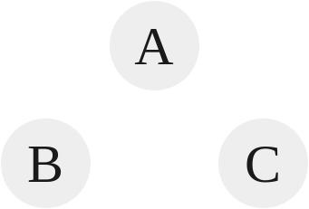
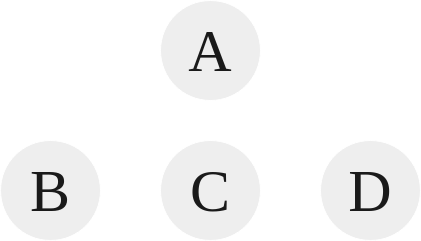
A tree is a rooted, directed, and acyclic in nature. In other words, it has a single root, each node has a single parent, and there are no cycles.

Tree 1

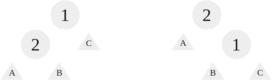
Tree 1 is an example of a basic valid tree. The root of this tree is A, and each node has a single parent. B’s parent is A, and C’s parent is also A. In this way, B and C are referred to as siblings. The parent are the predecessor of a node, while children are the successor of a node. Tree’s aren’t necessarily limited to just two children though. For instance, look at the following tree:

Tree 2

In the case of Tree 2, there is a single root, A, and A has three children B, C, and D. Every node has either a single parent or no parent.

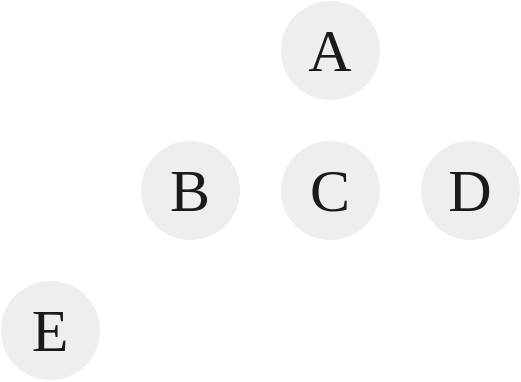
Tree 3

Dissecting Tree 3:

• E is the grandparent of A.

• E’s ancestors are B and A. B’s ancestors is A only.

• A’s descendants is every node underneath it, so B, C, D, and E. B’s descendants are E. C, D, and E have no descendants (nor children.)

• C, D, and E are leaf nodes or external nodes. These are nodes that have no children.

• B and A are non-leaf nodes or internal nodes because they possess children.

• A possesses three subtrees. A subtree of a node is a tree whose root is a child of that node. So the three subtrees of A are B and E, C, and D. B possess one subtree, E. E, C, and D possess zero subtree.

• The level or depth of this tree is 2. The level of a node is the distance of that node from the root. The root, A, is on level zero. B, C, and D are on level one. E is on level two. To compute the level of a tree, where $n$ is a node:

  • $\text{if } n \text{ is root:}$
    • $\text{level}(n) = 0$
  • $\text{else:}$
    • $\text{level}(n) = \text{level(parent)} + 1$

• The height of a tree is the number of nodes in the longest path from the root node to a leaf node. In this case, the height of this tree is 3, as the longest path contains 3 nodes, A, B, and E. To compute the height of a tree:

  • $\text{if the tree has just a root}$
    • $\text{Height = 1}$
  • $\text{else:}$
    • $\text{Height} = \text{max(Height(children))} + 1$

There are quite a few use cases for trees, such as Family Tress, Decision/Logic Trees, File Systems, Expression Trees, and Searching Trees.

N-Ary Trees

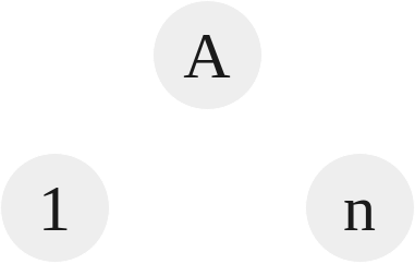
Tree 4

• A tree with each node consisting of at maximum $n$ children.
• The tree has three properties:
  1. Single root.
  2. Each node has a single parent.
  3. No cycles.

In this example above, we see that the root A has $1..n$ children. So if $n = 3$, each node can have at max 3 children.

Binary Trees

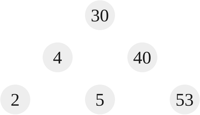
Tree 5

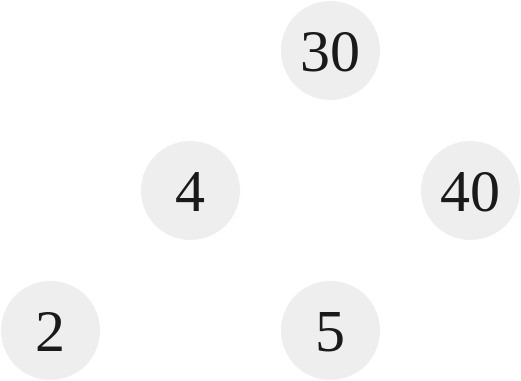
A binary tree is a tree with each node consisting of at most 2 children. In the above tree, Tree 5, notice that every node branches to at max 2 children. The root node, 30, as well as 4, branch off to two children, 40 branches to one element. 2, 5, and 53 branch off to zero children.

A binary tree node would look something like:

1
2
3
4
5
6
7
8

class TreeNode
{
  public:
    int value;
    TreeNode* left;
    TreeNode* right;
    TreeNode(int x) : value(x), left(nullptr), right(nullptr) {} 
}

Full Binary Tree

Tree 6

Tree 6 here is a full binary tree. That means that every node has either 2 children or 0 children.

Perfect Binary Tree

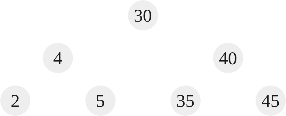
Tree 7

Tree 7 is a perfect binary tree. That means that given a height $h$ of the tree, the number of nodes contained is exactly $2^h - 1$. The height, $h$, of Tree 6 and Tree 7 is 3. The number of nodes contained in Tree 6 is 5. The number of nodes contained in Tree 7 is 7. Thus, for Tree 6:

$$2^h - 1 = 2^3 - 1 = 7 \ne 5$$

By this formula, a perfect binary tree node count for this height would be 7, but in the case of Tree 6, the count is 5 which means it is not a perfect binary tree. Looking at Tree 7:

$$2^h - 1 = 2^3 - 1 = 7 \equiv 7$$

Because our node count for Tree 7 is 7, it is a perfect binary tree.

It should be noted that if a tree is perfect, it’s height is $O(\log n)$, where $n$ is the number of nodes.

Complete Binary Tree

A complete binary tree is a tree which is perfect through levels $n - 1$, with some extra leaf nodes at level $n$ (height of the tree), all towards the left. In other words, for a tree at level $n$, there should be nodes filling each space from the left to the right, but it doesn’t need to fill all the way towards the right.

To illustrate, Tree 5 isn’t a complete binary tree. This is because it goes from left to right on the bottom most level, 2, 4, and 53. To make it complete, 40 must have a left child. Tree 6 is in fact a complete binary tree. This is because from left to right, it goes 2 and 4. 40 might not have any children, but there aren’t any gaps between the siblings of the bottom level, thus making it complete. This means that Tree 6 is both complete and full. A perfect binary tree like Tree 7 is also complete and full. Every perfect binary tree is complete and full, but not every complete and full binary tree is a perfect binary tree.

Binary Search Tree

A binary search tree is a tree in which every node’s left descendants are less than the current node’s value and every node’s right descendants are larger than the current value. A binary search tree is an ordered binary tree. Tree 5-7 have all be binary search trees. For instance, in Tree 5 the root is 30, to the left is 4, less than 30, and to the right is 40, greater than 30. We notice that every value to the left of 30 is less than it, e.g. 2,4,5. Conversely, every value to the right of 30 is greater than it, e.g. 40, 53.

Binary Search Tree Operations

The TreeNode class above can be used to create an insert method and search method for a BST:

 1
 2
 3
 4
 5
 6
 7
 8
 9
10
11
12
13
14
15
16
17
18
19
20
21
22
23

TreeNode* insert(TreeNode* root, int key)
{
  if (root == nullptr) 
    return new TreeNode(key); // Base case, this is where the value
                              // should be inserted
  if (key < root->value)      // key is less than current value
    root->left = insert(root->left, key);
  else if (key > root->value) // key is greater than the current value
    root->right = insert(root->right, key);
  
  return root;                // travel back up the stack
}

TreeNode* search(TreeNode* root, int key)
{
  if (root == nullptr || root->value == key) // Either have found the node
    return root;                             // or deemed it doesn't exist

  if (key < root->value)                     // check the left as it is <
    return search(root->left, key);
  
  return search(root->right, key);           // check the right as it is >
}

We can see the use of recursion when dealing with trees, using branches to access different elements. This principle is useful when dealing with trees. Unlike insert and search, the method deleteNode is a bit more complicated. Here is what the method looks like:

 1
 2
 3
 4
 5
 6
 7
 8
 9
10
11
12
13
14
15
16
17
18
19
20
21
22
23
24
25
26
27
28
29
30
31
32
33
34
35
36
37
38
39
40
41
42
43
44

TreeNode* deleteNode(TreeNode* root, int key)
{
  if (root == nullptr) // node doesn't exist
    return root;

  if (key < root->value) // search for key to the left
    root->left = deleteNode(root->left, key);
  else if (key > root->value) // search for key to the right
    root->right = deleteNode(root->right, key);
  else // found the node
  {
    // This is the case that there is no children
    if (root->left == nullptr and root->right == nullptr) 
    {
      delete root;
      return nullptr;
    }
    else if (root->left == nullptr) // child exists to the right
    {
      TreeNode* temp = root->right;
      delete root;
      return temp;
    }
    else if (root->right == nullptr) // child exists to the left
    {
      TreeNode* temp = root->left;
      delete root;
      return temp;
    }

    // both children exists
    TreeNode* current_node = root->right;

    // search for the lowest value to the right
    while (current_node && current_node->left != nullptr)
      current_node = current_node->left;

    // set the current value to be deleted to the lowest value
    root->value = current_node->value;
    // delete the lowest value found
    root->right = deleteNode(root->right, current_node->value);
  }
  return root;
}

If we are wanting to delete a node, we not only have to find it, but also have to consider a few cases:

1. Deleting a node with no children.

   • In this case, we just delete the data and return nullptr. This can be seen on lines 12-17.

2. Deleting a node with one child.

   • In this case, we need to delete the data and then set the node to be either the left or the right, given what is present. This can be seen on lines 18-29.

3. Deleting a node with two children.

   • In this case, it can be a bit hard to understand what we are supposed to do. The thing that must be understood is that the left values are always less than the current node, and the right values are always greater than the current node. What we can do is search for the least greatest value on the right side. This is guaranteed to be larger than the left, but also less than the right. After we find this value, we can just set the current node that we want to delete to this value, and then do a delete operation on the right tree on this value. This effectively just swaps the values, and then we continue forward to delete more. This can be seen on lines 31-41.

Traversals

A traversal is a method that “looks at” or “touches” every element in the data structure. In the context of a BST, that means that it visits every node in a tree. There are two different types of traversals:

• Depth First Strategy (DFS)
  • In a DFS method, the algorithm starts at the root node and then explores as far as possible along each branch before back tracking. There are 3 different types of methods that we’ll look over for this:
    • Inorder
    • Preorder
    • Postorder
• Breadth First Strategy (BFS)
  • In a BFS method, the algorithm looks at all the nodes at a current depth before going onto the next depth (or level.) This is contrast to DFS which will go as deep as it can for each branch. We’ll look at only one BFS:
    • Levelorder

A search and a traversal are similar but they are not the same. With a search, it isn’t always necessary to visit every element in the list. In contrast, a traversal always requires every node to be visited.

Inorder

The inorder traversal is literally what it sounds like, it is inorder. The strategy for an inorder traversal is:

1. Visit the left subtree
2. Visit the current node (root)
3. Visit the right subtree

The inorder method looks like this:

 1
 2
 3
 4
 5
 6
 7
 8
 9
10
11
12
13

#include <iostream>

void inorder(TreeNode* head)
{
  if (head == nullptr)
    std::cout << "";
  else
  {
    inorder(head->left);             // print everything to the left, <
    std::cout << head->value << " "; // print current value
    inorder(head->right);            // print everything to the right, >
  }
}

The inorder of Tree 7 is $2, 4, 5, 30, 35, 40, 45$.

Preorder

The preorder traversal is like the inorder but the steps are:

1. Visit the current node (root)
2. Visit the left subtree
3. Visit the right subtree

The preorder method looks like this:

 1
 2
 3
 4
 5
 6
 7
 8
 9
10
11
12
13

#include <iostream>

void preorder(TreeNode* head)
{
  if (head == nullptr)
    std::cout << "";
  else
  {
    std::cout << head->value << " "; // print current value
    preorder(head->left);            // print everything to the left, <
    preorder(head->right);           // print everything to the right, >
  }
}

The preorder of Tree 7 is $30, 4, 2, 5, 40, 35, 45$.

Postorder

The postorder traversal is like the preorder but the steps are:

1. Visit the left subtree
2. Visit the right subtree
3. Visit the current node (root)

The postorder method looks like this:

 1
 2
 3
 4
 5
 6
 7
 8
 9
10
11
12
13

#include <iostream>

void postorder(TreeNode* head)
{
  if (head == nullptr)
    std::cout << "";
  else
  {
    postorder(head->left);            // print everything to the left, <
    postorder(head->right);           // print everything to the right, >
    std::cout << head->value << " ";  // print current value
  }
}

The postorder of Tree 7 is $2, 5, 4, 35, 45, 40, 30$.

Levelorder

The levelorder traversal is a lot different than the rest because it is a BFS not a DFS traversal. The general idea is to traversal all nodes in level 0 up to level $n - 1$, where $n$ is the height of the tree. This can be done with queues:

 1
 2
 3
 4
 5
 6
 7
 8
 9
10
11
12
13
14
15
16
17
18
19
20
21
22
23
24

#include <iostream>
#include <queue>

void levelorder(TreeNode* root)
{
  std::queue<TreeNode*> node_queue;
  node_queue.push(root);

  while (!node_queue.empty())
  {
    TreeNode* temp = node_queue.front();
    node_queue.pop();
    if (temp)
    {
      if (temp->left)
        node_queue.push(temp->left);
    
      if (temp->right)
        node_queue.push(temp->right);

      std::cout << temp->value << " ";
    }
  }
}

In this method, we basically are breaking down the tree each level. We start with the root being queued, the loop immediately dequeues it, then inserts the left and right elements into the queue, and then prints the root. Next loop iteration does the same thing, but if we notice because it is a queue, it dequeues the left, queues its children, dequeues the right, queues its children. It perfectly travels level by level.

The levelorder traversal of Tree 7 is $30, 4, 40, 2, 5, 35, 45$.

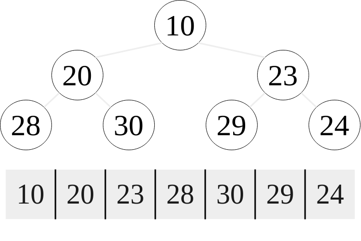
Tree Representation

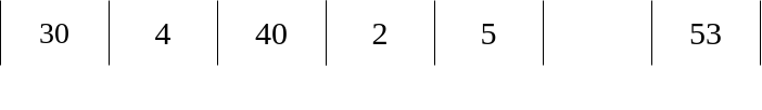
An array representation of Tree 5

Previous examples of trees used a node based design, where nodes contained pointers to children nodes. This is called a linked representation. Technically there are other ways to do it. One such way is an array representation. In an array representation, each element in the array represents an element in the tree. Given $i$ being the index of the array, the left child of an element is $2i + 1$, and the right child of an element is $2i + 2$. This array pictured above represents the same tree as Tree 5. The disadvantage of this method is wasted memory. In the case of the children of $40$, we can see that a right child is present, $45$, but there is an empty space at index $5$. Another disadvantage is the fact that there is a finite amount of space for a tree. An advantage is random access is now possible.

Operation Performance

When considering the time complexities of these operations, it is important to consider the characteristics of a binary search tree. When we think of a perfect tree, it must be noted that the maximum number of nodes in a tree is $n = 2^{h-1}$. The minimum number of nodes in a tree is $n = h$, as we can see below in Tree 8. Thus, the number of nodes falls in the range $h \le n \le 2^{h-1}$. Inversely, the height of the tree falls between $(\text{ceil}(\log (n+1)) - 1) \le h \le n -1$. The operations time complexity is at worst $O(h)$, where $h$ is the height of the tree. When considering how $h$ grows with $n$, we must consider the difference between balanced and unbalanced trees. A balanced tree is a tree in which the left and right subtrees of every node differ in their height by no more than 1. For the most part, the trees we have considered are pretty balanced. There height is approximately $\log n$. However, consider a tree like the following:

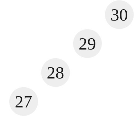
Tree 8

We can see how in this tree, every parent has only one node. This is called a degenerate tree and in this case, the $h = n$. Thus, for a balanced tree the worst case time complexity of the above operations are $O(\log n)$ and for an unbalanced tree the worst case time complexity is $O(n)$. The best case for these operations is $O(1)$, where the element is found either found at the root node or can be inserted right after the root node. Note that the time complexity for a traversal is always $O(n)$, this is because a traversal visits every node in the tree. When can we say a tree is balanced or unbalanced? Trees that are considered either only non-full or full can be considered unbalanced. Trees that are perfect or complete can be considered balanced. Please note that a full tree can be balanced though. If you are told that a tree is full though with no further information, it is safe to assume that it can be unbalanced, and its worst case time complexity for the operations above should be described as $O(n)$. This means that for optimal performance, we want a tree that is as balanced as possible, or as perfect as possible. Surmising things, an operation takes $O(h)$, but $h$ can be proportional the elements, $n$, depending on the structure of the tree. We want the height to grow with $\log n$, not with $n$, for optimal performance.

Insertion Permutations & The Catalan Number

When inserting a set of individual elements into a tree, there are $n!$ number of combinations that can be generated. The different unique combinations of binary trees that can be generated with a set of nodes is called the Catalan number. This can be calculated with the following, where $n$ is the number of nodes being inserted:

$\displaystyle C_n = \frac{1}{n+1}(\begin{smallmatrix}2n \ n\end{smallmatrix}) = \frac{(2n)!}{(n+1)!n!}= \prod_{k=2}^n \frac{n+k}{k}$

So, when the $n$ nodes is equal to 1, the Catalan number is 1, when it is 2, the Catalan number is 2, when it is 3, the Catalan number is 5, etc. etc.

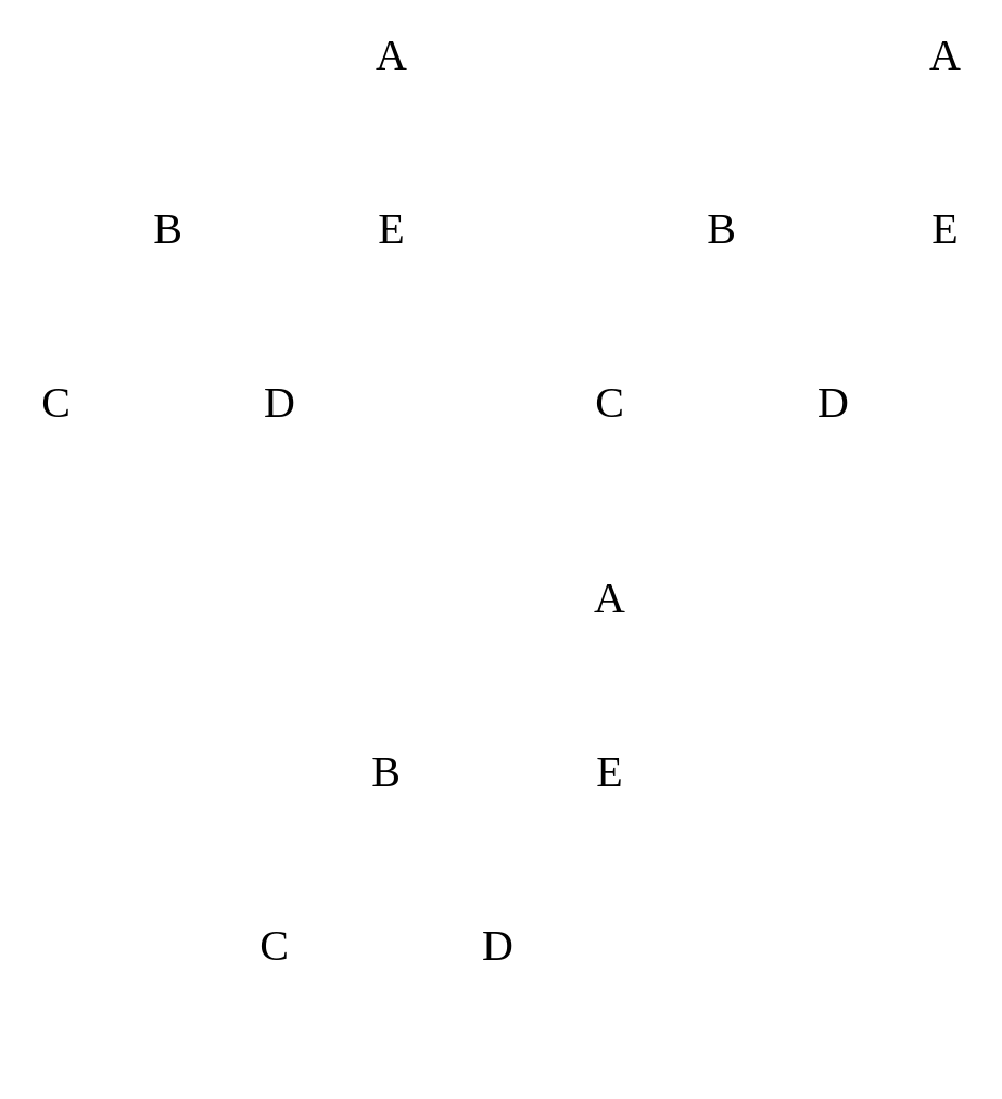
Rotations

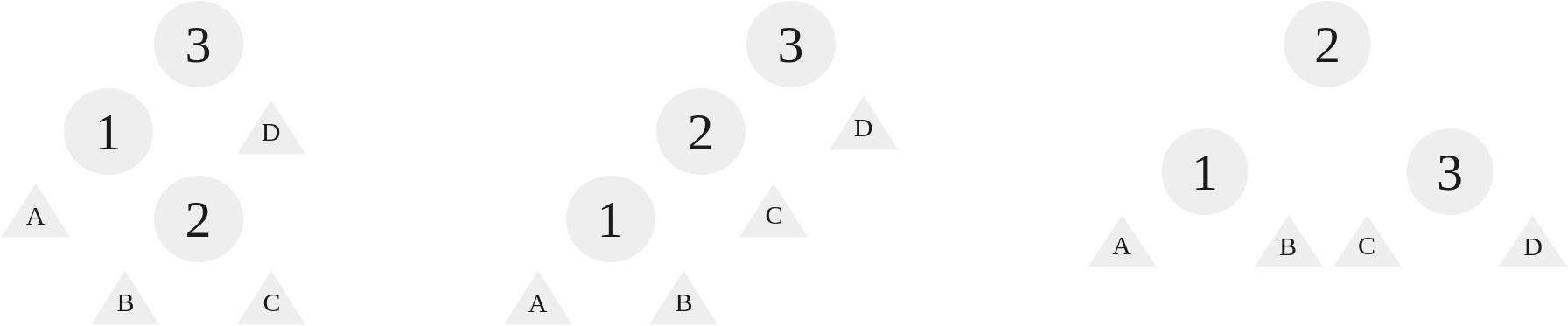
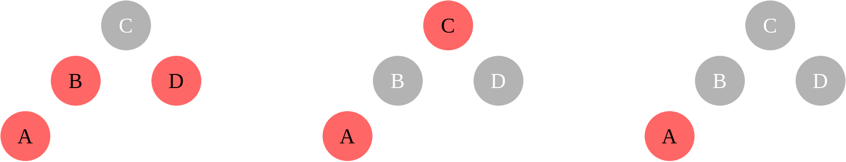
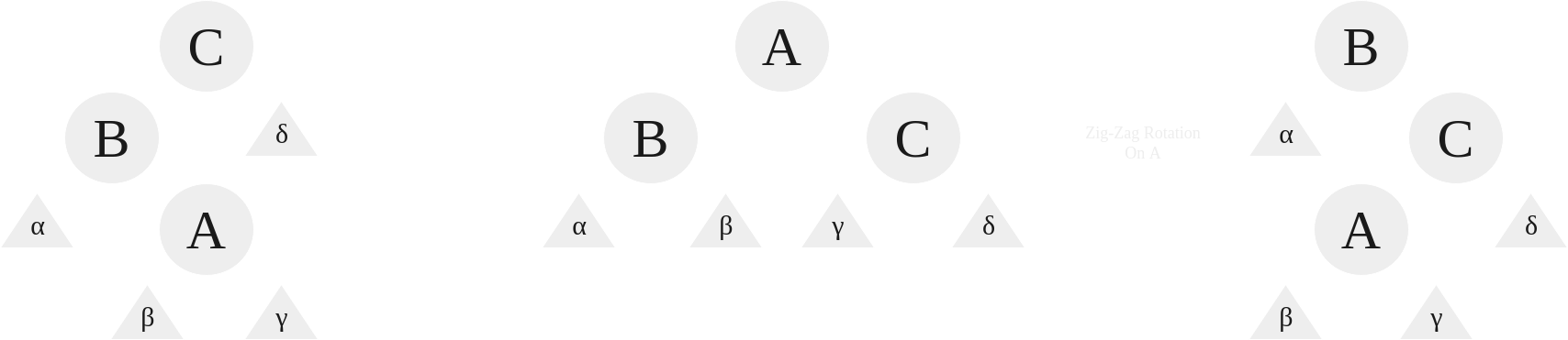
Given the performance benefits of having a tree that is more balanced, when we have a tree like Tree 8 it is in our best interest to perform a rotation. A rotation a is a tool that can be used to rearrange the tree without affecting its semantics (i.e. it doesn’t break the rules.) These rotations all take $O(1)$ time. Imagine for a moment we are given a set of nodes, $N$, such that $N = \lbrace1,2,3\rbrace$. The Catalan Number $C_3 = 5$, so there are 5 unique combinations for this set of nodes:

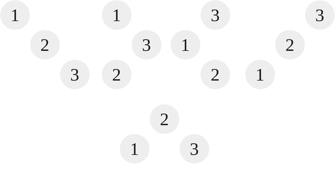
Combinations of a 3,2,1 BST

As we can see from above, out of the five possible combinations, only the final tree is balanced, that being the $\lbrace2,3,1\rbrace$ or $\lbrace2,1,3\rbrace$ tree. The rest are unbalanced. The goal of a rotation is to turn the four other trees into that fifth tree. This means that rotations only operate on 3 nodes at a time. They are used recursively to operate on an entire tree. There are four different types of rotations, and we will demonstrate them on each individual tree above, showing how we can convert the tree into the balanced fifth tree.

Left Rotation: RR Case

When the nodes are structured right, right, we use a left rotation. With a left rotation, we rotate the root to the left, making the root’s right child the new root:

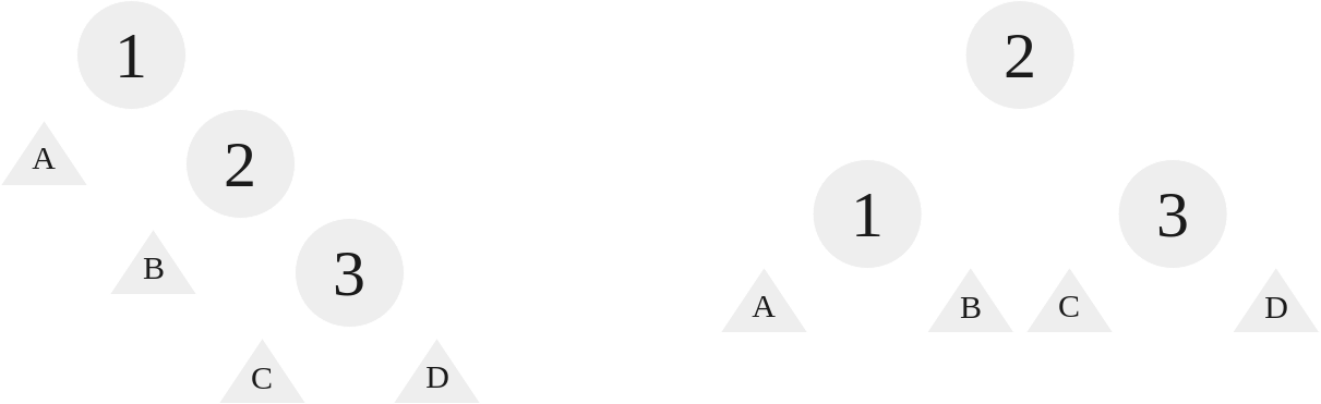
A left rotation on the RR case

As we can see, for these three nodes, we “grab” 2 and let 1 and 3 hang from it, setting 1’s right to 2’s left. The triangles represent branches, their size and contents arbitrary, they can be empty for all we care, they just need to be accounted for in the algorithm.

Right Rotation: LL Case

When the nodes are structured left, left, we use a right rotation. With a right rotation, we rotate the root to the right, making the root’s left child the new root:

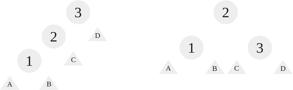
A right rotation on the LL case

Like before, we kind of “grab” 2 and 1 and 3 hang, but we set 3’s left to be 2’s right.

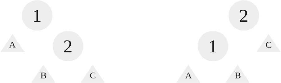
Right Left Rotation: RL Case

When the nodes are structured right, left, we use a right left rotation. With a right left rotation, we rotate at the right element, 3, and then at the root element, 1:

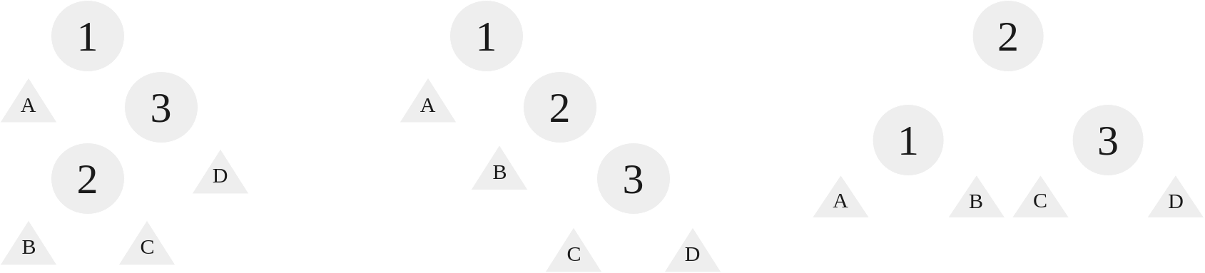
A right left rotation on the RL case

As we can see, this case requires two rotations. First, a right rotation on 3 such that 3 is now the right child of 2, inheriting the right child of 2. Afterwards, we perform a left rotation on 1, and this follows just like the other left rotation as outlined earlier.

Left Right Rotation: LR Case

When the nodes are structured as left, right, we use a left right rotation. With a left right rotation, we rotate at left element, 1, and then at the root element, 3:

A left right rotation on the LR case

As we can see, this case requires two rotations, similar to RL rotation. First, a left rotation on 1 such that 1 is now the left child of 2. Afterwards, we perform a right rotation on 3, and this follows just like the other right rotation as outlined earlier.

The Issue With Rotations

Rotations are great, but the issue is that for prebuilt BST trees using these rotations is very impractical. Utilizing these rotations in an unbalanced tree to make them balanced is hard, and it is much wiser to use what is called an AVL Tree to get this done.

AVL Trees

An AVL Tree is named after its inventors, Adelson-Velsky and Landis. It is a self-balancing binary search tree, meaning that it is designed to keep its height small. AVL tree’s are just a fancy binary tree when considering its properties. What it possesses is what is called a balance factor. The balance factor is a number that each node possesses that speaks about the height difference between its left and right children. Thus, for a node $n$, the balance factor $\text{BF}(n) = \text{Height(Left Child)} - \text{Height(Right Child)}$. A Binary Tree is an AVL tree if the invariant $\text{BF}(n) \in \lbrace-1,0,1\rbrace$ is true for ever node, $n$, in the tree. Here is an example of an AVL tree:

AVL Tree 1

As we can see, to the right of each Node is this balance factor. How do we implement an AVL Tree node? It is identical to the other node, but instead we include a height variable:

1
2
3
4
5
6
7
8
9

class AVLTreeNode
{
  public:
    int value;
    int height;
    AVLTreeNode* left;
    AVLTreeNode* right;
    AVLTreeNode(int x, int h) : value(x), height(h), left(nullptr), right(nullptr) {} 
};

When do we know when to balance? Well, using our definition before of the balance factor, $\text{BF}(n)$, we can use our previous rotations discussed on the AVL tree as we’re inserting. The cases to change are as follows:

In the case that $\text{BF}(n)$ is defined instead as $\text{BF}(n) = \text{Height(Right Child)} - \text{Height(Left Child)}$, which is common, just reverse the signs here. This means that because the rotations as discussed earlier are $O(1)$, the cost to insert, delete, and search is just the height of the tree, and because the height is maintained around $\log n$, this means that the worst and average case performance for these operations is $O(\log n)$.

AVL Tree Operations and Time Complexity

For search, AVL Tree’s operate the same as a BST. For insertion and deletion though, this is a bit different. After an insertion and deletion, the height of all the nodes in the search path might change, and as a result if the balance factor rule is broken, we rotate from the deepest node that breaks the balance factor rule up the search path. The search path is important to understand. If we insert on the right subtree and not on the left, it makes no sense to check the left for any adjustments in the balance factor, because it wasn’t effected. These rotations earlier are basically the same, but depending on the implementation height adjustments may have to be made. Because AVL Trees are heavily used in the coursework for COP3530, any code associated with them has been removed. The time complexity for these operations is as follows:

This is because the height of the AVL Tree, $h$, grows with $\log n$, as it is balanced. This means that all of these operations are $O(h)$, just like a BST, but because this AVL tree is balanced, $O(h) = O(\log n)$.

Red-Black Trees

A red-black tree is a binary search tree with one extra bit that dictates its “color,” either red or black. These colors are used to constrain the path these nodes can take, ensuring that no path is greater than twice the length as any other. This means that it is approximately balanced. An example red-black tree node would be:

 1
 2
 3
 4
 5
 6
 7
 8
 9
10
11

struct RedBlackTreeNode
{
	int value;
	RedBlackTreeNode* parent; // pointer to parent, a nullptr
	RedBlackTreeNode* left;   // if the parent doesn't exist
	RedBlackTreeNode* right;
	bool color; // true -> red, false -> black

  RedBlackTreeNode(int value) : value(value), parent(nullptr),
  left(nullptr), right(nullptr), color(true) {}
};

To maintain balance, a red-black tree must maintain the following properties:

1. Every node is either red or black.
2. The root must be black.
3. Every leaf (nullptr) must be black.
4. If a node’s color is red, its children must be black.
5. For every node, each path from the current node to its leaves must contain the same number of black nodes.

An example of a red-black tree is as follows:

Red-Black Tree 1

Every node is either red or black, fulfilling property one. As we can see, the root node is 30, and it is black, fulfilling property two. 30’s children are black, and the grandchildren of 30 are red. The leaf nodes are included, these are all nullptr and black, this fulfills property three. Because the leaf nodes are considered black and red’s children are black, this fulfills property four. Each path from root contains 3 black nodes inclusive, 2 black nodes exclusive. In other words, if we include the root every path from the root contains 3 black nodes (leaf nodes considered) and if don’t include the root every path from the root contains 2 black nodes (leaf nodes considered.) The red nodes do not count towards this path consideration. Each exclusive path is included to the right of each node. Notice that the paths from any node includes the same number of black nodes. This fulfills property five.

Rotations

Red-Black trees are a little different than AVL rotations.

Red-Black Tree Left Rotation

 1
 2
 3
 4
 5
 6
 7
 8
 9
10
11
12
13
14

void RedBlackTree::leftRotate(RedBlackTreeNode* element)
{
  RedBlackTreeNode* rchild = element->right;
  element->right = rchild->left;
  rchild->left = element;
  rchild->parent = element->parent;
  if (!rchild->parent)
    this->root = rchild;
  else if (element == element->parent->left)
    element->parent->left = rchild;
  else
    element->parent->right = rchild;
  element->parent = rchild;
}

Red-Black Tree Right Rotation

 1
 2
 3
 4
 5
 6
 7
 8
 9
10
11
12
13
14

void RedBlackTree::rightRotate(RedBlackTreeNode* element)
{
  RedBlackTreeNode* lchild = element->left;
  element->left = lchild->right;
  lchild->right = element;
  lchild->parent = element->parent;
  if (!element->parent)
    this->root = lchild;
  else if (element == element->parent->left)
    element->parent->left = lchild;
  else
    element->parent->right = lchild;
  element->parent = lchild;
}

Insertion

When we insert a node, its color is set to red. If the parent is also red, this will break some rules, so we need to test for some cases. In the event that the parent and the uncle of the node is red, that falls into case 1 which means we need to set the uncle and parent to black, and the grandparent to red. In the event that the parent is the left (right) child of the grandparent and the inserted node is the right (left) child of the parent, then we need to perform a left (right) rotation on the parent, that falls into case 2. Finally in the event that the parent is the left (right) child of the grandparent and the inserted node is the left (right) child of the parent, then we need to set the parent to black, grandparent to red, and then perform a right (left) rotation on the grandparent. Here are some visualizations for these cases:

• Case 1, Element’s uncle is red

Insertion Case 1

• Case 2, Element’s uncle is black and element is a right child and Case 3, element’s uncle is black and element is a left child.

Insertion Case 2 & 3

Here is a possible implementation the insert operation inspired from Cormen’s pseudocode:

 1
 2
 3
 4
 5
 6
 7
 8
 9
10
11
12
13
14
15
16
17
18
19
20
21
22
23
24
25
26
27
28
29
30
31
32
33
34
35
36
37
38
39
40
41
42
43
44
45
46
47
48
49
50
51
52
53
54
55
56
57
58
59
60
61
62
63
64
65
66
67
68
69
70
71
72
73
74
75
76
77
78
79
80
81
82
83
84

bool insert(int element)
{
  RedBlackTreeNode* y = nullptr; // leaf node
  RedBlackTreeNode* x = this->root;
  while (x != nullptr) // determine leaf node to insert at
  {
    y = x;
    if (element < x->value)
      x = x->left;
    else
      x = x->right;
  }

  RedBlackTreeNode* newNode = new RedBlackTreeNode(element);
  newNode->parent = y;
  if (y == nullptr)            // empty tree
    this->root = newNode;
  else if (element < y->value) // insert new node to left
    y->left = newNode;
  else if (element > y->value) // insert new node to right
    y->right = newNode;
  else                         // duplicate node
    return false;              // couldn't be inserted

  fixInsertTree(newNode);
  return true;                 // successful insert
}

void fixInsertTree(RedBlackTreeNode* element)
{
  while (element->parent && element->parent->color == true) // while parent is red
  {
    RedBlackTreeNode* grandparent = element->parent->parent;
    if (element->parent == grandparent->left) // parent is left child
    {
      RedBlackTreeNode* rightUncle = grandparent->right;
      if (rightUncle && rightUncle->color == true) // Case 1
      {
        element->parent->color = false;
        rightUncle->color = false;
        grandparent->color = true;
        if (grandparent == this->root) { break; }
        element = grandparent;
      }
      else 
      {
        if (element == element->parent->right)     // Case 2
        {
          element = element->parent;
          leftRotate(element);    // LR = Left rotate
        }                                        
        element->parent->color = false;            // Case 3
        grandparent->color = true;
        rightRotate(grandparent); // LL = Right rotate
        element = element->parent;
      }
    }
    else // parent is right child
    {
      RedBlackTreeNode* leftUncle = grandparent->left;
      if (leftUncle && leftUncle->color == true) // Case 1
      {
        element->parent->color = false;
        leftUncle->color = false;
        grandparent->color = true;
        if (grandparent == this->root) { break; }
        element = grandparent;
      }
      else 
      {
        if (element == element->parent->left)    // Case 2
        {
          element = element->parent;
          rightRotate(element);  // RL = Right rotate
        }                                        
        element->parent->color = false;          // Case 3
        grandparent->color = true;
        leftRotate(grandparent); // RR = Left rotate
        element = element->parent;
      }
    }
  }
  this->root->color = false;
}

For the sake of the course work and such, I won’t go over the deletion here. It is a similar method though, check out the Red-Black Tree chapter in “Introduction to Algorithms” for a deep dive into it.

Operation Performance

The operation performance for Red-Black trees is identical to AVL Trees.

The explanation also being the same, these trees are balanced, all operations are $O(h)$, and because $h$ grows with $\log n$, $O(h) = O(\log n)$.

Splay Trees

Splay trees are a unique balanced tree that allows faster access to previous accessed elements. To do this, special rotations are used.

Rotations

• The Zig Rotation

The zig rotation is the simplest rotation, and it is identical to the rotations described in the Red-Black Tree. As such, they will be skipped.

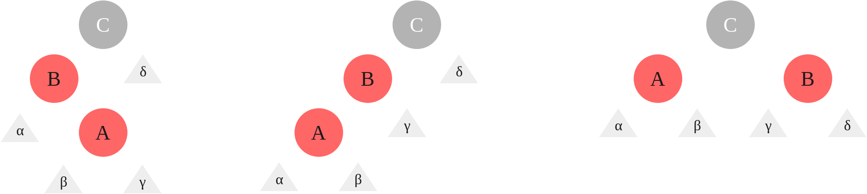
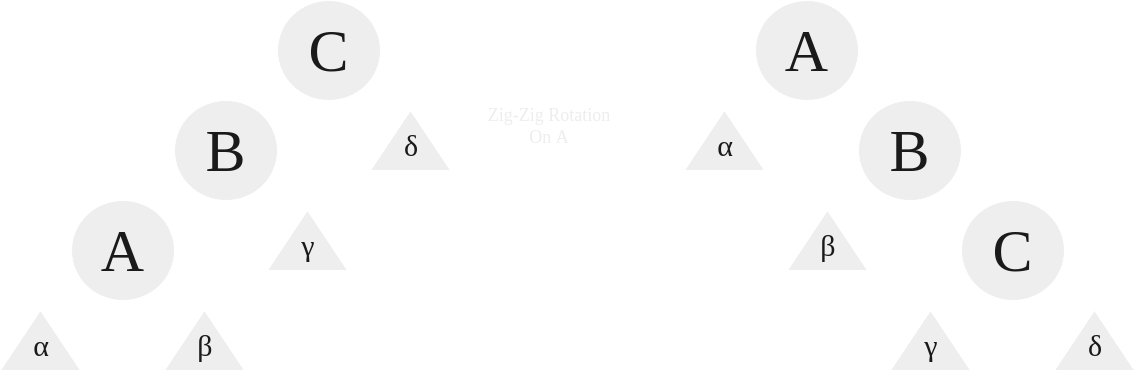
• The Zig-Zig and Zag-Zag Rotation

The Zig-Zig is the case where a splayed node is the left child of a left child, and the Zag-Zag is the case where a splayed node is the right child of a right child.

Zig-Zig and Zag-Zag Rotation

• The Zig-Zag Rotation

The Zig Zag case is when the splayed node is the left child of a right child or vice-versa.

Zig-Zag Rotation

Operation Performance

The time-complexity of a splay tree averages at $O(\log n)$ but at worst is $O(n)$.

Though the worst case is $O(n)$, subsequent operations are faster, and for repeated duplicate lookups (e.g. searching for the number “5” 30 times in a row) incredibly quick. These trees are mainly used in Cache and Garbage Collection applications.

B Trees

In B Trees, each “node” is a block containing at most $l$ keys. So when $l = 4$, the node can contain 1 value or 4 values, but not 5. Also, a B Tree can have at maximum $n$ children. Let’s go over the properties of a B tree with this knowledge. The maximum number of keys in a tree given its height $h$ (assuming the height of a root with no children is 0, thus this is a 0-indexed height), its maximum children $n$, and its maximum key count $l$ is:

$$\displaystyle ln^h + (n-1) \sum_{a=0}^{h-1}(n^a) = ln^h+n^h - 1$$

If a tree’s height is instead 1-indexed, meaning that a root with no children’s height is instead defined as 1, the formula is instead:

$$\displaystyle ln^{h - 1} + (n-1) \sum_{a=0}^{h-2}(n^a) = ln^{h-1}+n^{h-1}-1$$

• Property 1

Each node is a block containing multiple “keys,” where the maximum number of keys is $l$.

• Property 2

Each node can have at max $n$ children. In the case $n = 2$ and $l = 1$, that is just a BST.

• Property 3

B Trees are n-ary trees and they follow the BST property of everything on the left of a node is lesser, and everything on the right is greater. There can also be “middle” values, where these values fall between the minimum and the maximum. To visualize this, see the following:

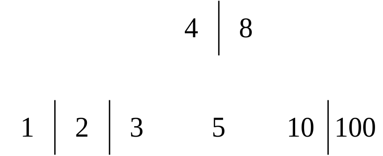
A B Tree where $n = 3$

• Property 4

If after an assertion a node’s key count is greater than $l$, then a node must be split. To do this, a tree is built from the bottom up. This split operation can be visualized here where $l = 4$:

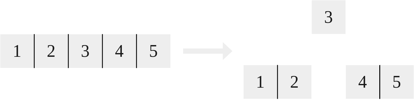
A B Tree split where $l = 4$

• Property 5

Leaf nodes are always at the same depth

• Property 6

A non-leaf node with $k$ children contains at most $k - 1$ keys. Leaf nodes have $[l / 2, l]$ keys and the maximum number of keys is no more than $n - 1$.

• Property 7

If root is a leaf, it has $0$ children, otherwise it has $[2, n]$ children. Internal nodes have $[\text{ceil}(n/2), n]$ children.

Insertion

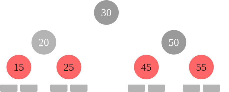
For insertion, keys are added to a node until they reach $l + 1$, at which they are split. The middle value is chosen as the new root. For instance, when $l = 3$, and we are using 1-indexes, key number 2 would be chosen. This is because there are 4 values in the node, which means the max index is 4, and because this is even, the “middle” value chosen is 2. So, the index chosen to split is $\text{ceil}((l + 1) / 2)$. Let’s take a look at an example where $l = 2$ and $n = 3$:

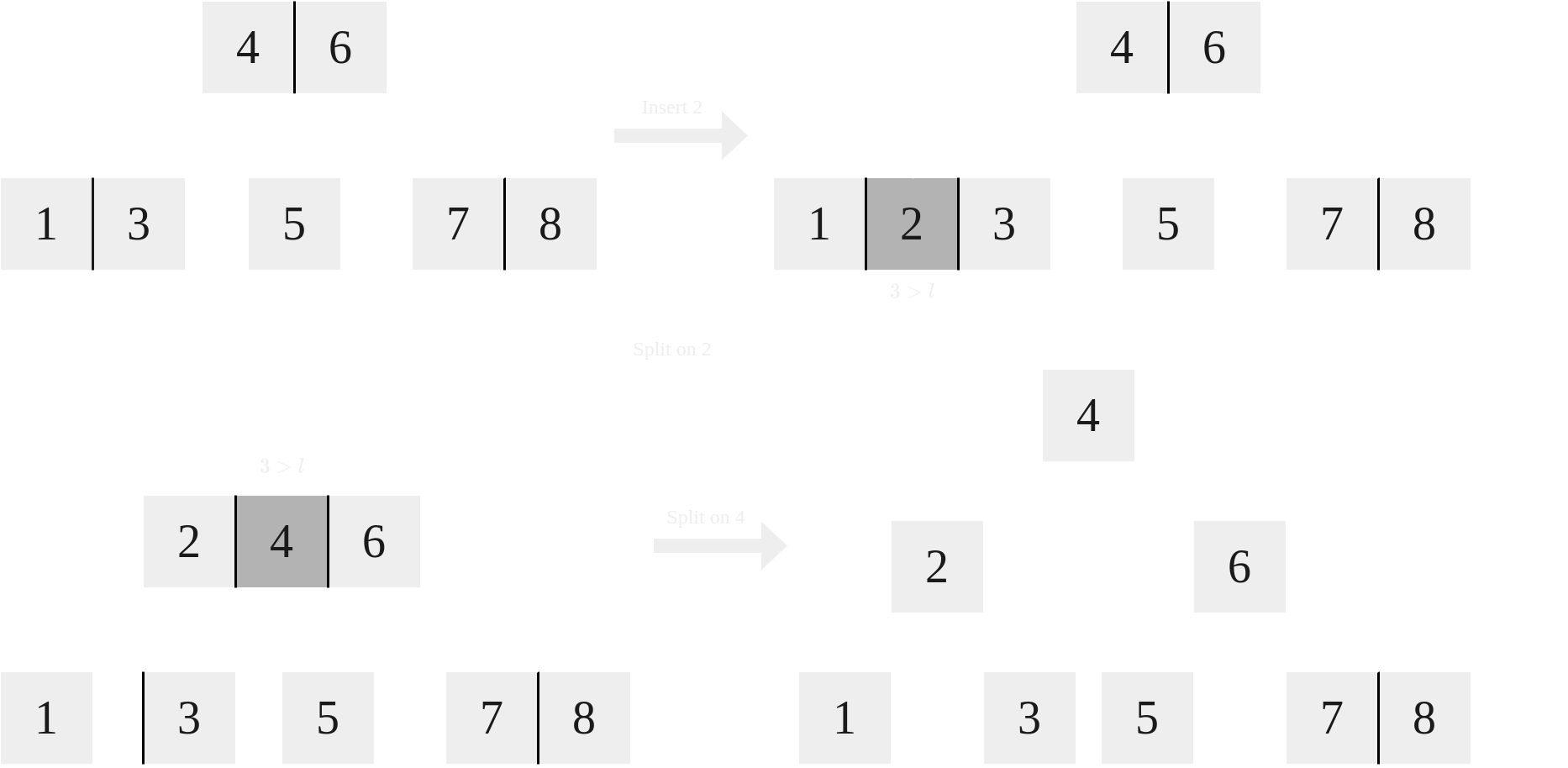
Inserting element 2 where $l = 4$ and $n = 3$

Operation Performance

Similar to Red-Black and AVL Trees, B trees are self balancing. The average and worst case for major operations is $O(\log n)$.

B+ Trees

In B+ Trees, the leaves contain all of the keys. Copies of the keys are held above the leaves. Also, the leaf nodes contain pointers to other leaves, forming a linked list. They have the added benefit for applications like hard drives, databases, etc. where data must be accessed at a specific point but more has to be accessed. The maximum number of values in a B+ tree given the height $h$ starting at 0, max number of children $n$, and max number of keys per node $l$, is $ln^h$. If a height is instead starting at 1, the formula is $ln^{h-1}$.

Operation Performance

Same as B trees.

Heaps

Motivation for a Heap and ADT

Imagine that we are designing a queue system. Within this system, people are given a number that corresponds to their position. Imagine also that we are nepotistic, and instead of favoring a “first come, first serve” model, we instead offer lower numbers (closer to the front of the queue) to those that we actually like. This idea is called a “priority queue.” It isn’t FIFO like a normal queue, but instead elements are assigned a priority and elements come out of the queue based on their priority. So the priority queue would keep track of highest or lowest priority item in a very fast way. The ADT for this would look like:

• Insert(element, priority) - Insert an element with a priority.
• ExtractMinimum() or ExtractMaximum() - Extract an element with minimum or maximum priority.

See, an implementation of a priority queue might be an unsorted array, and in the case of a minimum priority queue, insertion would be $O(1)$ because we’d just insert at the end of an array, but extraction would be $O(n)$, because we’d have to find the minimum most element in the entire array, then shift everything. What about a sorted array? Well, we’re just trading the times, now insertion is $O(n)$ and extraction $O(1)$, also not good. Same goes for a sorted list. Instead, we can use a binary heap, which has an insertion and extraction time complexity of $O(\log n)$.

Binary Heap

A Binary Heap is a complete binary tree, where every node is less than its children for a min heap and every node is greater than its children for a max heap. By that logic then, the root is the smallest element for a min heap and the largest for a max heap. Only the root can be removed. In this way, a heap Node looks something like this in a tree representation:

1
2
3
4
5
6

struct HeapNode
{
  int value;
  HeapNode* left;
  HeapNode* right;
}

Something to note though is the fact that we are dealing with a complete binary tree. This means that an array is actually very useful here. For a 0-indexed array, the root is at index 0, and the left child for a node at index $i$ is $2i+1$ and for a right child $2i+2$. Given a node at index $i$, its parent can be found with $\text{floor}((i - 1) / 2)$. Here is a representation of a binary heap as an array:

A binary min heap stored as an array visualized as a tree

Insertion (Heapify Up)

Assuming that we are using the array representation as before, when we insert an element it goes to the far left, the empty value:

Where To Insert an Element

Once we do that, we will calculate the parent with $\text{floor}((i - 1) / 2)$. Next, we run a while loop with the condition that the parent index is greater than or equal to 0 and that parent element is greater than the child element. In the loop, we swap the data held by the parent and the child, we set the child to be the parent, and then calculate the parent again. Here is this example for a min heap:

 1
 2
 3
 4
 5
 6
 7
 8
 9
10
11
12
13
14

#include <algorithm>

void insert(int value, int arr[], int lastElementIndex)
{
  arr[++lastElementIndex] = value;
  int child = lastElementIndex;
  int parent = (child - 1) / 2;
  while (parent >= 0 && arr[parent] > arr[child])
  {
    std::swap(arr[parent], arr[child]);
    child = parent;
    parent = (child - 1) / 2;
  }
}

The algorithm above minus the insertion part is heapify up. This is where the tree is “heapified” up the path. Insertion is $O(\log n)$.

Deletion (Heapify Down)

Deletion for a heap is removing the root node. To do this, we return the minimum value, and then delete it from the heap by swapping the last element in our array with the root. Afterwards, we compare the root to the children until it is in its proper place, swapping until then. The pseudocode would look something like this for a min heap:

 1
 2
 3
 4
 5
 6
 7
 8
 9
10
11
12
13
14
15
16
17
18
19
20

int returnRoot()
{
  int root = arr[0];
  arr[0] = arr[currentSize--];
  heapifyDown(arr, 0, currentSize);
}

void heapifyDown(int[] arr, int index, int size)
{
  1. if the left child & right child are >= size: return
  2. if left & right child are both smaller than the parent:
      if the left child is >= to the right child: 
        swap left child & parent, call heapify down on left child index: return
      else:
        swap right child & parent, call heapify down on right child index
  3. else if left child is >= to parent:
      swap left & parent, call heapify down on left child index
  4. else if right child is >= to parent:
      swap right & parent, call heapify down on right child index
}

Operation Complexity

In regards to the binary heap, the returnRoot/findMin/findMax operation is very very fast, and insert and delete are also very fast. Search with binary heap is slow, but this isn’t its primary purpose.

Graphs

Trees are hierarchical, acyclic, and have exactly one path between two nodes. Trees are a type of graph. Graphs don’t have to be hierarchy, they can be cyclic, and there can be multiple paths between one path and another. Graphs are basically an ordered pair of a set of vertices and a set of edges.

Terminology

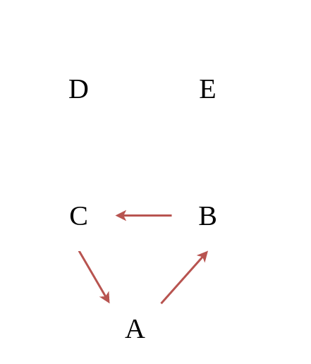
An example graph with terms

The vertex is a node in a graph. Vertices are a set, the set of vertices for the graph above are:

$$V = \lbrace A, B, C, D, E \rbrace$$

The number of vertices in a graph is given with $\vert V \vert$. In this case $\vert V \vert = 5$, as there are 5 elements.

The edge is a connection in a graph between two nodes. Edges are ordered pairs. The edges for the graph above are:

$$E = \lbrace \lparen A, B \rparen, \lparen B, B \rparen , \lparen B, C \rparen, \lparen C, A \rparen, \lparen C, D \rparen, \lparen D, E \rparen \rbrace $$

The number of edges in a graph is given with $\vert E \vert$. In this case, $\vert E \vert = 6$, because there are 6 elements. If you notice, one of the pairs is $\lparen B, B \rparen$, this indicates a self-loop. Simple graphs do not have self-loops. Self-loops are a “degenerate edge” and indicates that the graph above is a “pseudograph.”

The weight of an edge is an associated value of that edge. You can think of it as basically the cost to travel from one vertex to another over that edge.

Adjacent vertices is where a vertex is adjacent to another vertex if there is an edge to it from that other vertex. For example, C is adjacent to D, but D is not adjacent to C.

Simple graphs are graphs that don’t connect a vertex to itself (e.g. no self-loops) and there aren’t edges that connect the same vertices, i.e. no parallel edges. The graph above isn’t a simple graph, if you removed the loop, it would be a simple graph.

A path is a sequence of vertices in which each successive vertex is adjacent to its predecessor. For example, the path from A to D is A, B, C, D. The path from E to C doesn’t exist because E isn’t adjacent to D, and D isn’t adjacent to C. A simple path is one in which the path has no repeated vertices, except for the first and the last vertex.

A cycle is a simple path in which only the first and final vertices are the same. So, the path A, B, C, A is a cycle.

Connected vertex is when two vertices have a path between them. For example, A and E are connected, but E and D aren’t connected.

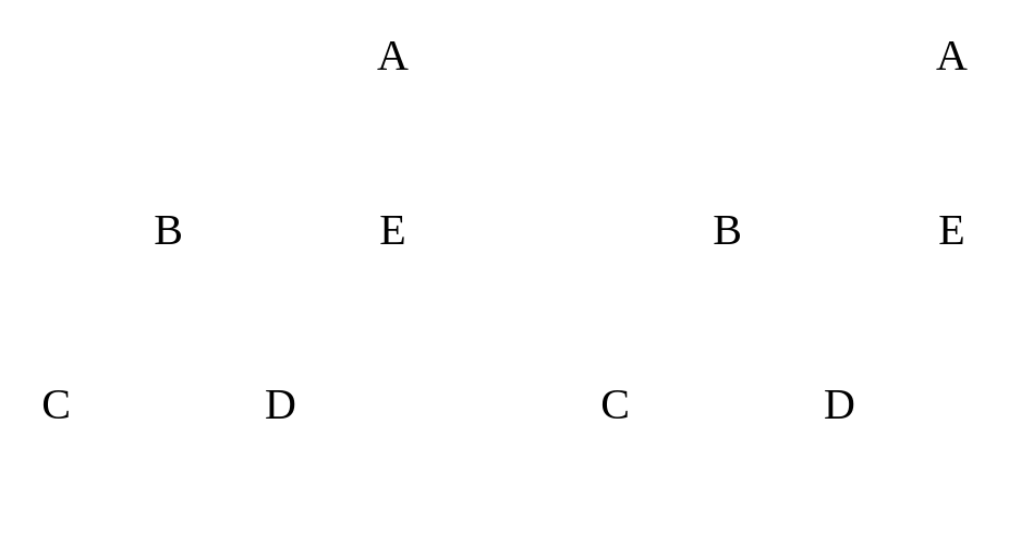
Types

Directed graph vs. Undirected graph

A directed graph (digraph) has directions of “flow.” This dictates things like paths and adjacency. An undirected graph is bidirectional. A directed graph can be converted into an undirected graph by duplicating any directional paths to a node, and then flipping its orientation.

Weighted graph vs. Unweighted graph

A weighted graph is a graph in which its edges carry a number that indicates a specific property. For instance, in the case of traffic indicators where each edge represents a street, these weights could represent the speed of getting through that specific path.

Connected graph vs. Not Connected graph

If we are given an undirected graph (a graph that doesn’t have arrow connectors, e.g. they aren’t one way, but both ways), it is a connected graph if there is a path from every vertex to every other vertex. This can be visualized by the following:

Cyclic graph vs. Acyclic graph

I defined cyclic above. Here are possible cyclic graphs for undirected and directed graph.

Dense graph vs. Sparse graph

When classifying graphs, we can assume that $\vert E \vert$ is $O(\vert V \vert^2)$ for a dense graph and $O(\vert V \vert)$ for a sparse graph. Sparse graphs have a small number of edges, close to $n$ where $n$ is the number of nodes, and for dense graphs they have a large number of edges, close to $n^2$. The actual minimums and maximums for each can be expressed as:

• Directed Graphs:

$$0 \le \vert E \vert \le (\vert V \vert)(\vert V \vert - 1)$$

• Undirected Graphs:

$$0 \le \vert E \vert \le \frac{(\vert V \vert)(\vert V \vert - 1)}{2}$$

Application of Graphs

Common examples of graph problems include:

• Social Networks, they utilize unweighted and undirected graphs.
• World Wide Web, they utilize unweighted and directed graphs.
• Maps, they utilize weighted and undirected graphs.

Common questions that can be answered with a graph include things like:

• Are there cycles in this path?
• What is the shortest route between points A and B?
• Is there a tour of this graph that uses each edge exactly once?

Implementation of Graphs

Graphs don’t really have an “ADT.” They existed before OOP. The API though must include graph methods and define how it should be used. The choices for this API have tradeoffs, and things we need to worry about is the runtime performance and the memory usage.

Nodes that are made with just labeled with letters or numbers are pretty useless. This is where the map data structure (see later for a description of that) comes into play. We can map a string to an int. E.g.

Common operations that are useful is determining the connectedness of two nodes, as well as the adjacency of nodes.

A One Graph API would look something like this:

 1
 2
 3
 4
 5
 6
 7
 8
 9
10
11
12
13
14
15
16
17
18
19
20
21
22
23
24
25

class Graph
{
  private:
    // Graph Implementation

  public:
    Graph();      // Graph constructor
    Graph(int V); // Construct Graph with vertex
    int V();      // Returns number of vertices
    int E();      // Returns number of edges

    void insertEdge(int from, int to, int weight);
    bool isEdge(int from, int to);
    int getWeight(int from, int to);
    std::vector<int> getAdjacent(int vertex);
    void printGraph();
}

class Path
{
  public:
    Path(Graph g, int s);
    bool hasPathTo(int s);
    std::vector<int> pathTo(int s);
}

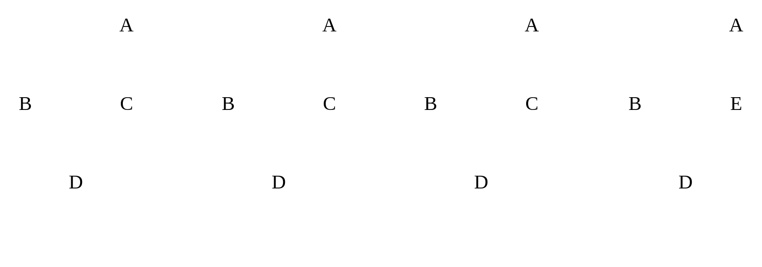
Edge List

An edge list just lists all the edges, and optionally gives the weight per edge. For example:

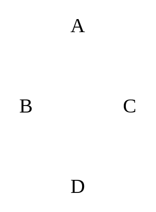
Example Graph with Weights

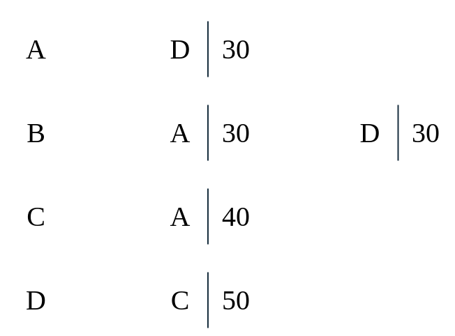
In the above example, we can draw out this as an edge list as the following:

The weights and adjacency here are completely arbitrary, but we can see the point. Common operations for an edge list are connectedness and adjacency, both of which are on average $O(E)$. The space taken up by an edge list implementation is also $O(E)$ on average, a well. At worst, all of these are $O(V^2)$.

Adjacency Matrix

An adjacency matrix is a way of representing adjacency. For the graph above, here is the matrix, where the rows represent from and the columns represent to:

If given a matrix, $M$, to insert a weighted element would be M[from][to] = weight, otherwise the default is M[from][to] = 0. If it unweighted, we would insert 1 if it is adjacent, 0 if it isn’t. The code to generate a matrix is the following:

 1
 2
 3
 4
 5
 6
 7
 8
 9
10
11
12
13
14
15
16
17
18
19
20
21
22
23
24
25

#include <iostream>
#include <map>
#include <string>
#define VERTICES 4;

int main()
{
  int no_lines, weight, j = 0;
  std::string from, to;
  int graph[VERTICES][VERTICES] = {0};
  std::map<std::string, int> mapper;

  std::cin >> no_lines;
  for (int i = 0; i < no_lines; i++)
  {
    std::cin >> from >> to >> weight;
    if (mapper.find(from) == mapper.end())
      mapper[from] = j++;
    if (mapper.find(to) == mapper.end())
      mapper[to] = j++;
    graph[mapper[from]][mapper[to]] = weight;
  }

  return 0;
} 

The time complexity to determine connectedness is $O(1)$. The time complexity to determine adjacency is $O(\vert V \vert)$. The space is $O(\vert V \vert^2)$.

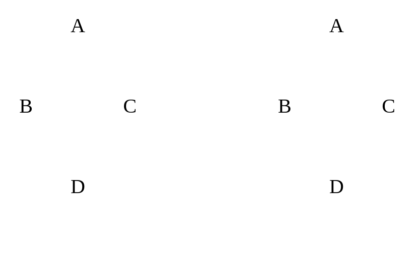
Adjacency List

The Adjacency Matrix has its pros, its cons though is that its space is massive. To alleviate this, an adjacency list can be utilized. An adjacency list is effectively a map, with each key pointing to a vector containing the adjacent vertices, and if weighted, its weight. A possible object to represent this would be like this:

1

std::map<int, std::vector<std::pair<int, int>>>

This is a map that stores ints as keys, and vectors of pairs of ints as values. The vector stores pairs because the first element is the vertex and the second element is the weight of the edge. To illustrate, this is the adjacency list of the graph above:

Example of Adjacency List

As you can see, unlike an edge list, each individual vertex has a list, and this list then can be accessed. The time complexity for both connectedness and adjacency is $O(\text{outdegree}\vert V \vert)$. The outdegree is the number of edges which are going out of a vertex, $V$. The space is $O(\vert V \vert + \vert E \vert) \approx O(\vert V \vert)$. At worst it is $O(\vert V \vert^2)$. The implementation for this is as follows. In this implementation, each vertex is labeled as a string inside of an integer.

 1
 2
 3
 4
 5
 6
 7
 8
 9
10
11
12
13
14
15
16
17
18
19
20

#include <iostream>
#include <string>
#include <map>
#include <vector>
#include <iterator>

int main()
{
  int no_lines;
  std::string from, to, weight;
  std::map<std::string, std::vector<std::pair<std::string, int>>> graph;
  std::cin >> no_lines;
  for (int i = 0; i < no_lines; i++)
  {
    std::cin >> from >> to >> weight;
    graph[from].push_back(make_pair(to, std::stoi(weight)));
    if (graph.find(to) == graph.end())
      graph[to] = {};
  }
}

Graph Traversal

Because trees are just a sort of graph, the idea of having a traversals make sense for a graph as well. Just like trees, there are two types of searches, breadth first search and depth first search.

Breadth First Search

The pseudocode for the breadth first search is as follows:

• Take an arbitrary start vertex, mark it identified, and place it in a queue.
• while the queue is not empty
  • Take a vertex, $u$, out of the queue and visit $u$.
  • for all vertices, $v$, adjacent to this vertex, $u$
    • if $v$ has not been identified or visited
      • Mark it identified
      • Insert vertex $v$ into the queue.
  • We are now finished visiting $u$.

To mark if something has been identified, we can use an array of boolean values with the size $\vert V \vert$ to mark if they are true. Another implementation could use a map, with the vertex ID being the key, and the boolean indicating if it has been found or not as the value.

Depth First Search

The pseudocode for the depth first search is as follows:

• Take an arbitrary start vertex, mark it visited, and place it in a stack.
• while the stack is not empty
  • the item on the top of the stack is $u$.
  • if there is a vertex, $v$, which is adjacent to this vertex, $u$, that has not been visited
    • Mark $v$ as visited.
    • Push vertex $v$ onto the top of the stack.
  • else
    • Pop from the stack.

Just like the breadth first search, what we use to keep track of already searched for values is up to us, I prefer a map honestly.

Spanning Trees

Given a graph, a spanning tree is a subset of the edges such that there is only one edge connecting each vertex and all the verticies are connected. The tree must be connected and acyclic. The cost of the spanning tree is defined as the sum of the weights of the edges. The minimum spanning tree is the spanning tree with the smallest possible cost in weight. A spanning tree with $n$ vertices will have $n-1$ edges. Here are some possible, unweighted, spanning tree examples to visualize the point, the red edges represent the subset:

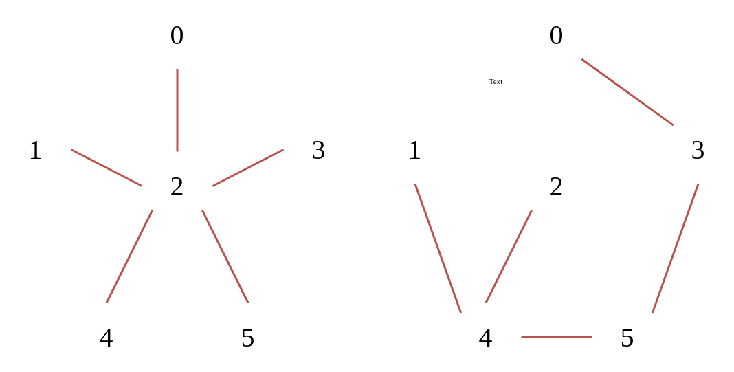
Examples of Spanning Trees

Graph Algorithms

s-t Path Algorithm

Given a graph, how can we figure out if there is a path between vertices $s$ and $t$? This isn’t asking what is the path, we are instead asking if there is a path. The easiest way to do this is to perform either a DFS or BFS on the vertex $s$ and if we ever encounter $t$, then we return true, else we return false.

Iterative Implementation

We can use an iterative implementation with a stack to determine the s-t path:

 1
 2
 3
 4
 5
 6
 7
 8
 9
10
11
12
13
14
15
16
17
18
19
20
21
22
23
24
25
26

#include <set>
#include <stack>

bool stPathDFS(const Graph& graph, int src, int dest)
{
  std::set<int> visited;
  std::stack<int> stk;
  visited.insert(src);
  stk.push(src);
  while(!stk.empty()) 
  {
    int z = stk.top();
    stk.pop();
    for (auto v: graph.adjList[u])
    {
      if (v == dest)
        return true;
      if ((visited.find(v) == visited.end()))
      {
        visited.insert(v);
        stk.push(v);
      }
    }
  }
  return false;
}

Recursive Implementation

Unlike the iterative implementation, we can instead use recursion:

 1
 2
 3
 4
 5
 6
 7
 8
 9
10
11
12
13
14
15
16
17
18
19
20
21
22
23
24

bool stPathDFSHelper(const Graph& graph, int src, int dest, std::vector<bool>& visited) 
{
  visited[src] = true;

  if (src == dest)
    return true;

  for (int neighbor: graph.adjList[src])
  {
    if (!visited[neighbor])
    {
      if (stPathDFSHelper(graph, neighbor, dest, visited))
        return true;
    }
  }

  return false;
}

bool stPathDFS(const Graph& graph, int src, int dest)
{
  std::vector<bool> visited(graph.numVertices);
  return stPathDFSHelper(graph, src, dest, visited);
}

Problems

Imagine that a graph is weighted. Say we want to figure out if A and C are connected. So, if we were to imagine this graph, say that there is a path from A to B, and then B to D, and then finally D to C. The weight from A to B is 10, the weight from B to D is 20, and the weight from D to C is 20. Imagine also another path from A to C exists, this being A to C directly with a weight of 25. A DFS would pick the A to B first on the basis of weight, and the path it would reveal would be A-B-D-C which has a weight of 50. A BFS would reveal this hidden path, so A-C would be chosen at 25, but imagine instead that the weight from A-C is 250, then A-B-D-C is indeed the path with the less weight. Other algorithm’s can figure this out. Some example algorithms include Dijkstra’s Algorithm, Bellman Ford Algorithm, Floyd-Warshall Algorithm, and A* Search Algorithm. We will be focusing on Dijkstra’s Algorithm and the Bellman Ford algorithm.

Dijkstra’s Algorithm

Dijkstra’s Algorithm allows us to find the shortest weighted path between two vertices. The characteristics are as follows:

• Single Source: Returns path to all vertices.
• Directed Graphs.
• No negative weights are allowed.
• No negative weight cycles allowed.
• Guaranteed to return a correct result if the edges are non-negative.
• Guaranteed to be optimal so long as there are no negative edges.
• It is a greedy algorithm.

There will be 4 data structures used to implement this algorithm, 2 arrays and 2 sets.

• Source vertex is called $s$
• Set $S$ will contain the vertices for which we have computed the shortest distance. $S$ at first will be empty.
• Set $V$ will contain all the vertices we still need to process. $V$ will be initialized with every vertex inside of it.
• Array $d$ will contain shortest distance from $s$ to some vertex, $v$. Initially all of $d$’s values will be set to infinity except for the $s$ index, which will be 0 (the path from source to source for a simple graph is 0.)
• Array $p$ will contain the predecessor of $v$ in the path from $s$ to $v$. This means that if the path from to $s$ to $v$ is $s$ to $a$ to $v$, $p \lbrack v \rbrack = a$. Initially all of $p$’s values will be set to -1.

Next comes the principle of relaxation. Relaxation is something I wish I had right now as I am studying for the final. Jokes aside, relaxation is the following formula:

• if dist[v] > dist[u] + weight(u, v)
  • dist[v] = dist[u] + weight(u, v)

This means for a vertex $v$ and a source vertex $s$, if the previous distance from $s$ to $v$ is greater than the distance from $s$ to $u$ plus the weight from $u$ to $v$, that means the weight of the previous path from $s$ to $v$ is greater than the current path of $s$ to $u$ to $v$.

With this in mind, we basically visit a vertex, relax its edges, and then visit the next vertex $v$ if $d \lbrack v \rbrack < d \lbrack \text{all other remaining vertices} \rbrack$, e.g. visit the next vertex with the least sized weight. While this is being done, we are updating array $p$ so that we are keeping track of the predecessors. After we have visited and computed every vertex, we return the paths. The idea behind returning the paths is actually quite ingenious. Imagine the following example graph, with a completed $d$ and $p$ arrays. Basically, this graph has had the algorithm run over it already:

Example Graph

Thus a table can be formed with the values generated by the algorithm:

So, the path from the source $s$, $0$, to $4$, would mean looking at $p\lbrack 4 \rbrack = 2$, then looking at $p\lbrack 2 \rbrack = 3$, etc. until we get to $s$, $0$. This means the path is $4 \to 2 \to 3 \to 0$.

Pseudocode

• Initialize set $S$ with the start vertex, $s$, and initialize set $V$ with the remaining vertices.
• for all $v$ in $V$
  • Set $p \lbrack v \rbrack$ to $s$
  • if there is an edge from $s$ to $v$
    • Set $d \lbrack v \rbrack$ to the weight($s, v$).
  • else
    • Set $d \lbrack v \rbrack$ to $\infin$
• while $V$ isn’t empty
  • for all $u$ in $V$, find the smallest $d \lbrack u \rbrack$.
  • Remove $u$ from $V$ and add $u$ to $S$.
  • for all $v$ adjacent to $u$ in $V$
    • if $d \lbrack v \rbrack > d \lbrack u \rbrack +$ weight($u, v$).
      • Set $d \lbrack v \rbrack$ to $d \lbrack u \rbrack +$ weight($u, v$).
      • Set $p \lbrack v \rbrack$ to $u$.

The time complexity of this pseudocode is $O(V \log V + V \log V + E \log V) = O(E \log V)$, assuming that $E > V$.

Prim’s Algorithm

In regards to a minimum spanning tree, what are some ways that we can algorithmically determine a minimum spanning tree? One such algorithm that solves this conundrum is Prim’s Algorithm. Prim’s Algorithm analyzes all the connections between vertices and finds the set with minimum total weight that makes the graph connected. The vertices thus are divided into two sets:

• $S$, the set of vertices in a spanning tree. This is initially empty.
• $V$, the remaining vertices, ones that aren’t in the spanning tree yet.

After this, the algorithm chooses the edge with the smallest weight that connects a vertex, $a$, in $S$ to a vertex $b$ in $V$, and then it adds it to the the minimum spanning tree by placing $b$ into $S$. The principle is quite easy, select a vertex, find the minimum weight, that is the edge to that vertex.

Pseudocode

• Input: An undirected, connected, weighted graph, $G$
• Output: $T$, a minimum spanning tree for $G$.
• $T \coloneqq \empty$.
• Pick any vertex in $G$ and add it to $T$.
• for $j = 1$ to $n - 1$, where $n$ is the number of vertices.
  • Let $C$ be the set of edges with one endpoint inside $T$ and one endpoint outside of $T$.
  • Let $e$ be a minimum weight edge in $C$ and $v$ be its associated endpoint vertex.
  • Add $e, v$ to $T$.

The time complexity Prim’s Algorithm is $O(EV)$, or $O(E \log V)$ if you utilize priority queues within the implementation.

Kruskal’s Algorithm

Unlike Prim’s Algorithm, Kruskal’s Algorithm can take directed and undirected edges. It’s approach is completely different. How the algorithm works is that it adds every possible edge to a list, and then sorts it in ascending order. Then a new minimum spanning tree is constructed from the list, avoiding any edges that generate a cycle. This rather straightforward up until here, how can we “detect” a cycle? One such method would be to utilize DFS, but its time complexity is very bad, its $O(E (V + E))$. A better method would be to use disjoint sets, or a “weighted union” sets. It consists of a group of sets, such that there is no item in common in any of the sets. This means that there are $n$ sets at first, each containing a vertex. From there, find and union set operations can take place, and a cycle can be detected. It stops whenever all the sets have been combined into one. For an operation called find($i$), which basically returns the set where an element $i$ exists, if for a given edge $i - j$:

• if find($i$) != find($j$) (if $i$ and $j$ don’t share the same set)
  • union($i, j$)

This simple method will always return a MST and its time complexity is $O(E \log V)$, much better than the DFS method.

Non-ordered Data Structures

Set ADT

A set is a collection that contains no duplicate elements. It is based on the mathematical set, e.g. a set $S = {3,1,4,9,2}$. Other sets are like sets of numbers, like the set of integer, $\Z$, or the set of real numbers, $\R$. A set object has the follow property:

1. They aren’t indexed.
2. They don’t reveal the order of insertion of items.
3. They enable efficient search and retrieval of information.
4. They allow removal of elements without moving other elements around.

The operations include:

1. find - Find an element in the set.
2. insert - Add an element to the set.
3. remove - Remove an element from the set.
4. union - Perform a set union operation between two sets, e.g. $A \cup B$.
5. intersection - Perform a set intersection operation between two sets, e.g. $A \cap B$.
6. difference - Perform a set difference operation between two sets, e.g. $A - B$.
7. subset - Return a subset.

The difference between sets and list are the following:

C++ Set

C++ contains two major set implementations:

Map ADT

A map is a collection of key-value pairs that doesn’t contain duplicate keys.

1. Maps are a kind of an abstraction over Sets
2. The Keys in a map are a Set.
3. Values can be non-unique (e.g. multiple values, unique keys)
4. If you store values along with keys in a Set data structure, you get a Map.

For instance a valid Map would be:

$$\lbrace(A, 1), (B, 5), (C, 1), (D, 6), …\rbrace$$

This is laid out such that it is (key, value). An invalid Map would be:

$$\lbrace(A, 1), (A, 5), (C, 1), (D, 6), …\rbrace$$

Some very simple examples of where a map is useful:

Maps in C++

Hash Table

We’ve learned the meaning of the Set and the Map. We can see that in the case of the C++ set and map, they are actually ordered. Why is that? Well this because they are built using Binary Search Trees. This makes the time complexity for most operations $O(\log n)$. This isn’t bad, but we can do better. This is where a hash table comes in. With a hash table we can get $O(1)$ access.

How? Well the idea isn’t terribly hard to understand. Imagine we have an array with 1, element, what is the access time to find the element at $A[0]$? The answer is $O(1)$. How about an array with 1,000,000 elements, and we want to access the 493,382 element, e.g. $A[493382]$? The answer is also $O(1)$. This idea behind constant lookup is very intuitive, notice though that to access data, we effectively use the following formula:

$$A[\text{key}] = \text{value}$$

This is very interesting, but has a fatal flaw, if memory doesn’t exist at this region, we’ll end up in trouble. Perhaps instead we can initialize everything with a default value. Say we create a boolean array:

1

bool[] set[100] = {0};

Now everything is false, and then when something exists at a specific index, we set it to true. This is cool, but what about other data types? Also that is a lot of wasted memory. One idea is to use something called hashing. For instance, imagine we have strings. How would we store “cat” or “dog?” Well we could convert “cat” or “dog” into a number, e.g. perhaps the first letter, c = 3, d = 4. Well that is cool, but what if we wanted to store “cap”? That is a collision. One way to get around this is by multiplying each letter by a power of 27. So cat turns into:

$$(3 \times 27^2) + (1 \times 27^1) + (20 \times 27^0) = 2234$$

This is our index. Because the base is always greater than or equal to 26, we are going to get a unique number and no collisions. Less than 26, we aren’t guaranteed no collisions by the pigeonhole principle. This works great for the alphabet. How about ASCII? That is 128 values. How about unicode? That is 143,859 values. Using this method is practically impossible. It’ll lead to overflows, which means collisions!

These hash codes have some issues, although cool. They can waste memory, and they still have collisions at their core. The solution? Allow for collisions but build it so that the algorithm resolves collisions and utilize small table sizes and then increase. This means that a number is reduced, e.g utilizing $%~10$ for example. This allows us to reduce the size of our table. So when given a key $2145$, we can do $2145~%~10 = 5$. This is fine and dandy buttt what if we do $25~%~10$… that is also 5. This is where utilize something called collision resolution. In the event an element already exists at a specific index, collision resolution is utilized. This is the idea behind a hash function.

Hash Functions

A hash function is a function that converts a data object into a hash code. Its properties include:

• Input: Object $x$
• Output: An integer representation of $x$
• If $x$ is equal to $y$, $H(x) = H(y)$
• If $x$ isn’t equal to $y$, it should mean $H(x) \ne H(y)$

So, a function that always returns 0 is technically a hash function, but a really bad one at that. A function returns the sum of the powers of 31 of an ASCII string is a much better hash function. A function that just returns a random number isn’t a hash function. Hash functions then usually utilize primes and smaller primes are preferred. Hash functions should be easy to compute, so smaller primes are faster to compute. So the hash functions spits out a number for a given input, it then puts it in the hash code, and then the hash code reduces the hash function output and resolves collisions. These are the different strategies for collision resolution:

• Open Hashing
  • Buckets
    • For a given index, multiple values could exist inside a bucket (doesn’t mean they have to though), basically acting as a linked list.
    • Load factor is a metric to show how full our hash table is. It is the number of elements divided by the number of buckets. For a load factor where buckets only store one element, the load factor has to be between $0 \le L \le 1$, where $L$ is the load factor. If a bucket can store more than one element, the load factor can be $L \ge 1$.
  • Separate Chaining
    • Fixed: This means that buckets can just grow, the linked list will keep going forward, this means that the time complexity will become $O(n)$, and that isn’t good. Instead, we can use the following resizable method.
    • Resizable: This is complicated to explain, but basically once the load factor exceeds a set amount, what you can do is double the number of buckets and double the reduce number, e.g. if the no. of buckets is 10, now it is 20, and if the reduce number is 10, it is now 20.
• Closed Hashing (Open Addressing)
  • The probing equation is defined as $h'(x) = (h(x) + f(i))$, where $x$ is our input, $i$ is an index being tested, $h(x)$ being our hash function, $f(i)$ being our probe. If the index revealed by $h'(x)$ already has an element present, increase $i$ by one and try again.
  • Linear probing: This is where if a spot is taken, it goes to the next available spot, and if a next available spot doesn’t exist, it jumps to the beginning of the storage container.
    • $f(i) = i$
  • Quadratic probing: This is similar to linear probing, but instead of jumping to the next spot, we jump to a spot following a specific sequence, for instance, $\lbrace1^2, 2^2, 3^3, …\rbrace$. This is more efficient than linear probing.
    • $f(i) = i^2$

Sorting

Data often has to be manipulated for it to be useful. One very useful manipulation you can do is sorting. Sorting is where an element, x, has a characteristic that can place it before or after another element, y. When a characteristic is determined, a sorting algorithm will take unsorted data and then place it in a specific order such that it can be traversed in order. For example:

$$\text{Unsorted: } \lbrace3, 1, 7, 2, 9…\rbrace \ \text{Sorted: } \lbrace1, 2, 3, 7, 9…\rbrace $$

There are a ton of sorting algorithms, some are better suited depending on the situation. The analysis of a sort will be based on this criteria to determine its situational efficiency:

1. Time Complexity
2. Space Complexity
3. Adaptive and/or Stable

Stable

Stable sorting algorithms preserve the relative order of equal elements. For example, imagine I have a list of student names with corresponding grades. Currently, the list is sorted alphabetically, but imagine I want to sort numerically. A stable sorting algorithm would not change the relative order of duplicates, thus a student with a first name A with a score of say 80 would be ahead of a student with a first name B with a score of 80. The use of a stable algorithm is that it makes it more efficient when there are duplicate cases, as we don’t have to sort by another key when a duplicate is present.

Adaptive

Adaptive sorting algorithms take advantage of existing order in its inputs, and this advantage makes it faster by not trying to reorder if it is already ordered. Bubble Sort and Insertion Sort are examples of adaptive sorting algorithms.

Quadratic Sorts

Selection Sort

Selection sort is an incredibly simple sort to understand. The premise as follows:

1. Find the smallest/largest element, $e_1$ in a collection of data, $C$.
2. Move this element, $e_1$, to its correct position.
3. Find the next smallest/largest element, $e_2$ in a $C$.
4. Move this element, $e_2$ to its correct position.
5. Repeat this process $\text{size}(C) - 1$ times.

The code follows like so:

 1
 2
 3
 4
 5
 6
 7
 8
 9
10
11
12
13
14
15
16

#include <algorithm>

void selectionSort(int[] arr, int size)
{
  for (int i = 0; i < size - 1; i++)
  {
    int min_pos = i;
    for (int j = i + 1; j < size; j++)
    {
      if (arr[j] < arr[min_pos])
        min_pos = j;
    }
    if (min_pos != i)
      std::swap(arr[min_pos], arr[i]);
  }
}

A visual of this for an array $\lbrace3, 1, 7, 2, 9, 4\rbrace$:

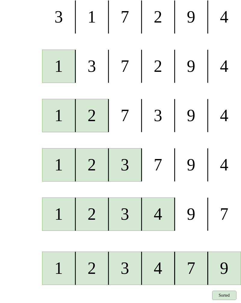
Example of Selection Sort

Bubble Sort

Bubble sort is also a very simple sort to understand. It is similar to selection sort, just a bit different. The premise is as follows:

1. Swap adjacent elements, $e_i$ and $e_{i+1}$, in a collection $C$ if they are out of order
2. Repeat swapping till you reach the end of the collection to bubble up the largest element after each iteration
3. Repeat this entire process $\text{size}(C) - 1$ times stopping at $\text{size}(C) - i$ after the $i^\text{th}$ iteration.

The code follows like so:

 1
 2
 3
 4
 5
 6
 7
 8
 9
10
11
12
13
14
15
16
17
18
19

void bubbleSort(int[] arr, int size)
{
  for (int i = 0; i < size - 1; i++)
  {
    bool swapped = false;
    for (int j = 0; j < size - 1 - 1; ++j)
    {
      if (arr[j] > arr[j + 1])
      {
        int temp = arr[j];
        arr[j] = arr[j + 1];
        arr[j + 1] = temp;
        swapped = true;
      }
    }
    if (!swapped)
      break;
  }
}

A visual of this for an array $\lbrace8,6,7,5,9,4\rbrace$:

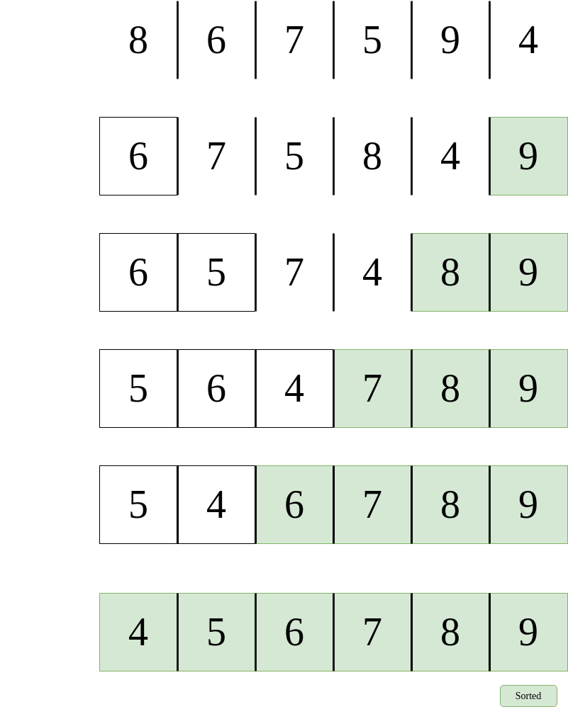
Example of Bubble Sort

Insertion Sort

Insertion sort is the last of the common quadratic sorts. It is probably the easiest one to understand. The premise is as follows:

1. Keep track of two regions, the Sorted region and the Unsorted region.
2. Initially, the sorted region will have one element.
3. Insert the first element in the unsorted region in the correct place of the sorted region.
4. Repeat this until there are no more elements in the unsorted region.

The code follows like so:

 1
 2
 3
 4
 5
 6
 7
 8
 9
10
11
12
13
14
15

void insertionSort(int[] arr, int size)
{
  for (int i = 1; i < size; i++)
  {
    int key = arr[i];
    int j = i - 1;

    while (key < arr[j] && j >= 0)
    {
      arr[j + 1] = arr[j];
      j--;
    }
    arr[j + 1] = key;
  }
}

A visual of this for an array $\lbrace8,6,7,5,9,4\rbrace$:

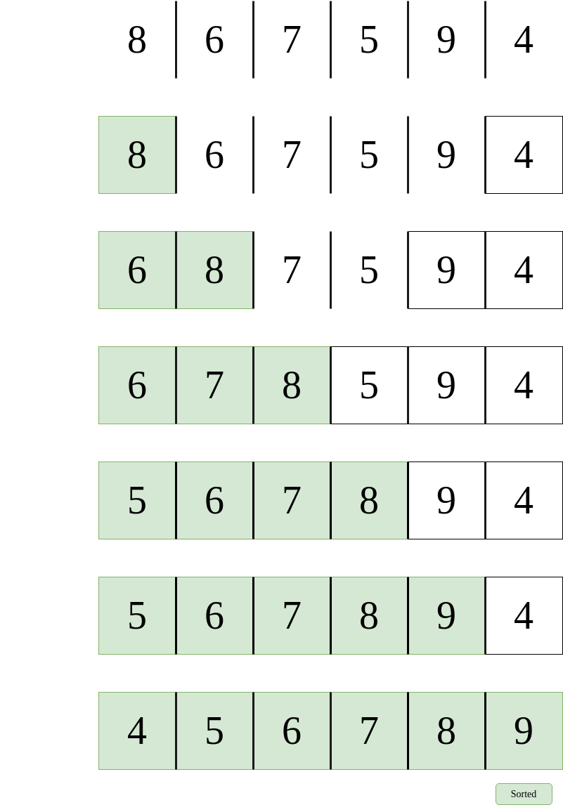
Example of Insertion Sort

Comparison

Shell Sort

Shell Sort is a modified version of Insertion Sort that is much more efficient. In this sort, things are divided into gaps, and then an insertion sort is conducted on each gap. The code for this looks like this:

 1
 2
 3
 4
 5
 6
 7
 8
 9
10
11
12
13
14
15
16
17
18

void shellSort(int[] arr, int size)
{
  for (int gap = size / 2; gap >= 1; gap /= 2)
  {
    for (int j = gap; j < size; j++)
    {
      int temp = arr[j];
      int i = j - gap;

      while (i >= 0 && arr[i] > temp)
      {
        arr[i + gap] = arr[i];
        i = i - gap;
      }
      arr[i + gap] = temp;
    }
  }
}

Performance

The performance of a shell sort is largely based on the sequence of decreasing values. For the power of 2 sequence as described above, performance is $O(n^2)$. For gaps based on Hibbard’s sequence, the performance is $O(n^\frac{3}{2})$.

Linearithmic

Merge Sort

Merge sort uses the property of divide and conquer. The premise is as follows:

1. Merge sort splits the array in half, sorts the two smaller halves, then merges the two sorted halves together.
2. Divide the array to be sorted subarrays till you reach a size 1.
3. In the conquer step, sort the two subarrays.
4. In the combine step, combine two sorted arrays.
5. Repeat this until you merge all elements in one array.

The code for this looks like this:

 1
 2
 3
 4
 5
 6
 7
 8
 9
10
11
12
13
14
15
16
17
18
19
20
21
22
23
24
25
26
27
28
29
30
31
32
33
34
35
36
37
38
39
40
41
42
43
44
45
46
47
48
49
50
51
52
53
54
55

void mergeSort(int[] arr, int low, int high)
{
  if (low < high)
  {
    int mid = low + (high - low) / 2;

    mergeSort(arr, low, mid);
    mergeSort(arr, mid + 1, high);

    merge(arr, low, mid, high);
  }
}

void merge(int[] arr, int low, int mid, int high)
{
  int x = mid - low + 1;
  int y = high - mid;

  int X[x], Y[y];

  for (int i = 0; i < x; i++)
    X[i] = arr[low + i];
  for (int j = 0; j < y; j++)
    Y[j] = arr[mid + low + j];

  int i = 0;
  int j = 0;
  int k = 1;
  while (i < x && j < y)
  {
    if (X[i] <= Y[j])
    {
      arr[k] = X[i];
      i++
    }
    else
    {
      arr[k] = Y[j];
      j++
    }
    k++;
  }
  while (i < x)
  {
    arr[k] = X[i];
    i++;
    k++;
  }
  while (j < y)
  {
    arr[k] = Y[j];
    j++;
    k++;
  }
}

Quick Sort

Quick Sort is similar to merge sort, but instead uses something called a pivot. The premise as follows:

1. Quicksort rearranges the array into two parts, called partitioning
2. A pivot is selected and the following is executed:
   1. All the elements in the left subarray are less than or equal to the pivot
   2. All the elements in the right subarray are larger than the pivot
3. Repeat this until the array is sorted.

The code for this looks like this:

 1
 2
 3
 4
 5
 6
 7
 8
 9
10
11
12
13
14
15
16
17
18
19
20
21
22
23
24
25
26
27
28
29
30
31
32
33
34
35
36
37
38

#include <algorithm>

void quickSort(int[] arr, int low, int high)
{
  if (low < high)
  {
    int pivot = partition(arr, low, high);
    quickSort(arr, low, pivot - 1);
    quickSort(arr, pivot + 1, high);
  }
}

int partition(int[] arr, int low, int high)
{
  int pivot = array[low];
  int up = low, down = high;

  while (up < down)
  {
    for (int j = up; j < high; j++)
    {
      if (arr[up] > pivot)
        break;
      up++;
    }
    for (int j = down; j > low; j--)
    {
      if (arr[down] < pivot)
        break;
      down--;
    }
    if (up < down)
      std::swap(arr[up], arr[down]);
  }

  std::swap(arr[low], arr[down]);
  return down;
}

Heap Sort

One of the interesting things we’ve covered is the heaps from earlier. One thing we can do is utilize a heap data structure, insert elements into the heap, then remove the elements from the heap and place it in the array. This comes out to be $O(n \log n)$.

Comparison

Matrices

Diagonal Matrix

A Diagonal Matrix is like the following:

    1 2 3 4 ...
1 | a 0 0 0
2 | 0 b 0 0
3 | 0 0 c 0
4 | 0 0 0 d
...

Which can be defined as $M[i, j] = 0 \text{ if } i \ne j$

This matrix will be the framework for later types of matrixes:

 1
 2
 3
 4
 5
 6
 7
 8
 9
10
11
12
13
14
15
16
17
18
19
20
21
22
23
24
25
26
27
28
29
30
31
32
33
34
35
36
37
38
39
40
41
42
43
44
45
46
47
48
49
50
51
52
53
54
55
56
57
58
59
60

#include <iostream>
class Matrix {
    private:
        int *A;
        int n;

    public:
        Matrix() {
            n = 2;
            A = new int [2];
        }

        Matrix(int n) {
            this->n = n;
            A = new int [n];
        }

        void Set(int i, int j, int x) {
            if (i == j) {
                A[i - 1] = x;
            }
        }

        int Get(int i, int j) {
            if (i == j) {
                return A[i - 1];
            }
            return 0;
        }

        void Display() {
            for (int i = 0; i < n; i++) {
                for (int j = 0; j < n; j++) {
                    if (i == j) {
                        std::cout << A[i] << " ";
                    } else {
                        std::cout << "0 ";
                    }
                }
                std::cout << std::endl;
            }
        }

        ~Matrix() {
            delete [] A;
        }
};

int main() {
    int size = 5;
    Matrix diagonal(size);

    for(int i = 1; i <= size; i++) {
        for(int j = 1; j <= size; j++) {
            diagonal.Set(i,j,i);
        }
    }

    diagonal.Display();
}

Returns:

1 0 0 0 0
0 2 0 0 0
0 0 3 0 0
0 0 0 4 0
0 0 0 0 5

Lower Triangle Matrix

A Lower Triangle Matrix is like the following:

    1 2 3 4 ...
1 | a 0 0 0
2 | b c 0 0
3 | d e f 0
4 | g h i j
...

Which can be defined as: $M[i, j] = 0 \text{ if } i < j$

$M[i, j] \ne 0 \text{ if } i \ge j$

When observing the space this matrix takes up, we can observe that each n row adds n amount of space, e.g.. 1 + 2 + 3, etc. etc. This means the number of non zero elements are give in $\frac{n(n+1)}{2}$, and the number of zero elements is given by $\frac{n(n-1)}{2}$.

Though this is the case, there are two methods to represent this as an array, the first is row major mapping:

A | 0 1 2 3 4 5 6 7 8 9
    a b c d e f g h i j

This corresponds to the rows in the first diagram. So 0 is the first row, 1 and 2 is the second, 3-5 the third, and 6-9 the fourth.

The second method is column major mapping:

    1 2 3 4 ...
1 | a 0 0 0
2 | b e 0 0
3 | c f h 0
4 | d g i j
...

So looking at our array now, 0-4 represents the first column, 5-6 represents the second column, 7 and 8 the third, and 9 the fourth.

Here is an implementation of Row Major mapping:

 1
 2
 3
 4
 5
 6
 7
 8
 9
10
11
12
13
14
15
16
17
18
19
20
21
22
23
24
25
26
27
28
29
30
31
32
33
34
35
36
37
38
39
40
41
42
43
44
45
46
47
48
49
50
51
52
53
54
55
56
57
58
59
60

#include <iostream>
class Triangle {
  private:
    int *A;
    int n;

  public:
    Triangle() {
      n = 2;
      A = new int [3];
    }

    Triangle(int n) {
      this->n = n;
      A = new int [n * (n + 1) / 2];
    }

    void Set(int i, int j, int x) {
      if (i >= j) {
          A[i * (i - 1) / 2 + j - 1] = x;
      }
    }

    int Get(int i, int j) {
      if (i >= j) {
        return A[i * (i - 1) / 2 + j - 1];
      }
      return 0;
    }

    void Display() {
      for (int i = 1; i <= n; i++) {
        for (int j = 1; j <= n; j++) {
          if (i >= j) {
            std::cout << A[i * (i - 1) / 2 + j - 1] << " ";
          } else {
            std::cout << "0 ";
          }
        }
        std::cout << std::endl;
      }
    }

    ~Triangle() {
      delete [] A;
    }
};

int main() {
    int size = 5;
    Triangle triangle(size);

    for(int i = 1; i <= size; i++) {
        for(int j = 1; j <= size; j++) {
            triangle.Set(i,j,i);
        }
    }

    triangle.Display();
}

Returns:

1 0 0 0 0
2 2 0 0 0
3 3 3 0 0
4 4 4 4 0
5 5 5 5 5

Upper Triangle Matrix

An Upper Triangle Matrix is represented as:

    1 2 3 4 ...
1 | a b c d
2 | 0 e f g
3 | 0 0 h i
4 | 0 0 0 j
...

Which can be defined as: $M[i, j] = 0 \text{ if } i > j$

$M[i, j] \ne 0 \text{ if } i \le j$

When observing the space this matrix takes up, we can observe that each n row adds n amount of space, e.g.. 1 + 2 + 3, etc. etc. This means the number of non zero elements are give in $\frac{n(n+1)}{2}$, and the number of zero elements is given by $\frac{n(n-1)}{2}$.

Like the Lower Triangle Matrix, there also exists a Column-Major Mapping, but we won’t get into that as the concept is basically the same. The implementation of this matrix is the same as the last, just adjust lines 19, 25, and 24 from i >= j to i <= j.

Symmetric Matrix

A Symmetric Matrix is represented as:

    1 2 3 4 ...
1 | a a a a
2 | a b b b
3 | a b c c
4 | a b c d
...

Which can be defined as:

$M[i,j] = M[j, i]$

This looks intimidating, but we already implemented this already, as if we notice, we can draw a diagonal line down the center, and anything to the right or to the bottom is already covered by the corresponding. Eg. we can represent this as either a Lower Triangle or an Upper Triangle, and just mirror it.

Tridiagonal Matrix

A Tridiagonal Matrix is represented as:

    1 2 3 4 5 ...
1 | a b 0 0 0
2 | c d e 0 0
3 | 0 f g h 0
4 | 0 0 i j k
5 | 0 0 0 l m
...

Which can be defined as:

$M[i, j] \ne 0 \text{ if } |i - j| \le 1$

Here is an implementation:

 1
 2
 3
 4
 5
 6
 7
 8
 9
10
11
12
13
14
15
16
17
18
19
20
21
22
23
24
25
26
27
28
29
30
31
32
33
34
35
36
37
38
39
40
41
42
43
44
45
46
47
48
49
50
51
52
53
54
55
56
57
58
59
60
61

#include <iostream>
#include <cmath>

class Triangle {
    private:
        int *A;
        int n;

    public:
        Triangle() {
            n = 2;
            A = new int [6];
        }

        Triangle(int n) {
            this->n = n;
            A = new int [3 * n];
        }

        void Set(int i, int j, int x) {
            if (abs(i - j) <= 1) {
                A[3 * i + abs(i - j)] = x;
            }
        }

        int Get(int i, int j) {
            if (abs(i - j) <= 1) {
                return A[3 * i + abs(i - j)];
            }
            return 0;
        }

        void Display() {
            for (int i = 1; i <= n; i++) {
                for (int j = 1; j <= n; j++) {
                    if (abs(i - j) <= 1) {
                        std::cout << A[3 * i + abs(i - j)] << " ";
                    } else {
                        std::cout << "0 ";
                    }
                }
                std::cout << std::endl;
            }
        }

        ~Triangle() {
            delete [] A;
        }
};

int main() {
    int size = 9;
    Triangle diagonal(size);
    for(int i = 1; i <= size; i++) {
        for(int j = 1; j <= size; j++) {
            diagonal.Set(i,j,i);
        }
    }

    diagonal.Display();
}

Result:

1 1 0 0 0 0 0 0 0
2 2 2 0 0 0 0 0 0
0 3 3 3 0 0 0 0 0
0 0 4 4 4 0 0 0 0
0 0 0 5 5 5 0 0 0
0 0 0 0 6 6 6 0 0
0 0 0 0 0 7 7 7 0
0 0 0 0 0 0 8 8 8
0 0 0 0 0 0 0 9 9

The formula for space is technically $3n -2$, but the space is basically ignorable so I just set it 3n.

Sparse Matrix

A sparse matrix is a matrix where non-zero elements can be anywhere in the matrix, such as:

    1 2 3 4 5 ...
1 | a 0 0 0 0
2 | 0 0 b 0 c
3 | d 0 e 0 0
4 | 0 f 0 0 0
5 | 0 0 0 g 0
...

As we can see, the elements are dispersed about the matrix, with no pattern. As a result, we have to store our elements using coordinates, namely their i and j coordinates. As a result, we can define the class Element to facilitate this:

1
2
3
4
5
6

class Element {
    public:
        int i;
        int j;
        int x;
};

Next, we need the actual Matrix, so we will use the class Sparse:

 1
 2
 3
 4
 5
 6
 7
 8
 9
10
11
12
13
14
15
16
17
18

class Sparse {
    private:
        int m; // Dimension
        int n; // Dimension
        int num; // Number of non-zero elements
        Element *ele; // Array of the elements.
    public:
        Sparse(int m, int n, int num) {
            this->m = m;
            this->n = n;
            this->num = num;
            ele = new Element[this->num];
        }

        ~Sparse() {
            delete[] ele;
        }
}

Next, we need a way to set and get the matrix, for this we are going to use the istream and ostream operators.

 1
 2
 3
 4
 5
 6
 7
 8
 9
10
11
12
13
14
15
16
17
18
19
20
21
22
23
24

friend std::istream & operator >> (std::istream &is, Sparse &s) {
    std::cout << "Enter non-zero elements ";
    for(int i = 0; i < s.num; i++) {
        std::cin >> s.ele[i].i >> s.ele[i].j >> s.ele[i].x; // Loop over
    }                                      // number of elements, assign
    std::cout << std::endl;
    return is;
}

friend std::ostream & operator << (std::ostream &os, Sparse &s) {
    int k = 0; // Current element
    for (int i = 0; i < s.m; i++) { // Go over the m coordinate
        for (int j = 0; j < s.n; j++) { // Go over the n coordinate
            if (s.ele[k].i == i && s.ele[k].j == j) {
                std::cout << s.ele[k++].x << " "; // increment k
            }
            else {
                std::cout << "0 ";
            }
        }
        std::cout << std::endl;
    }
    return os;
}

Last but not least, lets add a method to allow addition of two sparse matrices.

 1
 2
 3
 4
 5
 6
 7
 8
 9
10
11
12
13
14
15
16
17
18
19
20
21
22
23
24
25
26
27

Sparse operator+(Sparse &s) {
    if (m != s.m || n!=s.n) { // if the two arrays
        return Sparse(0, 0, 0); // dimensions do not match
    }
    Sparse *sum = new Sparse(m, n, num + s.num);

    int i, j, k;
    i = j = k = 0;
    while(i < num && j<s.num) {
        if (ele[i].i < s.ele[j].i) {
            sum->ele[k++] = ele[i++];
        } else if (ele[i].j > s.ele[j].j) {
            sum->ele[k++] = s.ele[j++];
        } else {
            sum->ele[k] = ele[i];
            sum->ele[k++].x = ele[i++].x + s.ele[j++].x;
        }
    }
    for(; i < num; i++) {
        sum->ele[k++] = ele[i];
    }
    for(; j < s.num; j++) {
        sum->ele[k++] = s.ele[j];
    }
    sum->num = k;
    return *sum;
}

Putting it all together:

 1
 2
 3
 4
 5
 6
 7
 8
 9
10
11
12
13
14
15
16
17
18
19
20
21
22
23
24
25
26
27
28
29
30
31
32
33
34
35
36
37
38
39
40
41
42
43
44
45
46
47
48
49
50
51
52
53
54
55
56
57
58
59
60
61
62
63
64
65
66
67
68
69
70
71
72
73
74
75
76
77
78
79
80
81
82
83
84
85
86
87
88
89
90
91
92
93
94
95

#include <iostream>
using namespace std;

class Element {
    public:
        int i;
        int j;
        int x;
};

class Sparse {
    private:
        int m; // Dimension
        int n; // Dimension
        int num; // Number of non-zero elements
        Element *ele; // Array of the elements.
    public:
        Sparse(int m, int n, int num) {
            this->m = m;
            this->n = n;
            this->num = num;
            ele = new Element[this->num];
        }

        friend istream & operator >> (istream &is, Sparse &s) {
            cout << "Enter non-zero elements ";
            for(int i = 0; i < s.num; i++) {
                cin >> s.ele[i].i >> s.ele[i].j >> s.ele[i].x;
            }
            cout << endl;
            return is;
        }

        friend ostream & operator << (ostream &os, Sparse &s) {
            int k = 0; // Current element
            for (int i = 0; i < s.m; i++) { // Go over m coordinate
                for (int j = 0; j < s.n; j++) { // Go over n coordinate
                    if (s.ele[k].i == i && s.ele[k].j == j) {
                        cout << s.ele[k++].x << " "; // increment k
                    }
                    else {
                        cout << "0 ";
                    }
                }
                cout << endl;
            }
            return os;
        }

        Sparse operator+(Sparse &s) {
            if (m != s.m || n!=s.n) { // if the two arrays
                return Sparse(0, 0, 0); // dimensions do not match
            }
            Sparse *sum = new Sparse(m, n, num + s.num);

            int i, j, k;
            i = j = k = 0;
            while(i < num && j<s.num) {
                if (ele[i].i < s.ele[j].i) {
                    sum->ele[k++] = ele[i++];
                } else if (ele[i].j > s.ele[j].j) {
                    sum->ele[k++] = s.ele[j++];
                } else {
                    sum->ele[k] = ele[i];
                    sum->ele[k++].x = ele[i++].x + s.ele[j++].x;
                }
            }
            for(; i < num; i++) {
                sum->ele[k++] = ele[i];
            }
            for(; j < s.num; j++) {
                sum->ele[k++] = s.ele[j];
            }
            sum->num = k;
            return *sum;
        }

        ~Sparse() {
            delete[] ele;
        }
};

int main() {
    Sparse s1(5,5,5);
    Sparse s2(5, 5, 5);
    cin >> s1;
    cin >> s2;

    Sparse sum = s1 + s2;

    cout << "S1" << endl << s1;
    cout << "S2" << endl << s2;
    cout << "Sum" << endl << sum;
    return 0;
}